Type:	Package
Title:	Fast Permutation Based Two Sample Tests
Version:	2.0.1
Description:	Fast randomization based two sample tests. Testing the hypothesis that two samples come from the same distribution using randomization to create p-values. Included tests are: Kolmogorov-Smirnov, Kuiper, Cramer-von Mises, Anderson-Darling, Wasserstein, and DTS. The default test (two_sample) is based on the DTS test statistic, as it is the most powerful, and thus most useful to most users. The DTS test statistic builds on the Wasserstein distance by using a weighting scheme like that of Anderson-Darling. See the companion paper at <doi:10.48550/arXiv.2007.01360> or https://codowd.com/public/DTS.pdf for details of that test statistic, and non-standard uses of the package (parallel for big N, weighted observations, one sample tests, etc). We also include the permutation scheme to make test building simple for others.
License:	GPL-2 | GPL-3 [expanded from: GPL (≥ 2)]
Encoding:	UTF-8
LinkingTo:	cpp11
RoxygenNote:	7.2.3
URL:	https://twosampletest.com, https://github.com/cdowd/twosamples
BugReports:	https://github.com/cdowd/twosamples/issues
Suggests:	testthat (≥ 3.0.0)
Config/testthat/edition:	3
NeedsCompilation:	yes
Packaged:	2023-06-23 18:50:48 UTC; cdowd
Author:	Connor Dowd [aut, cre]
Maintainer:	Connor Dowd <cd@codowd.com>
Repository:	CRAN
Date/Publication:	2023-06-23 19:30:02 UTC

Anderson-Darling Test

Description

A two-sample test based on the Anderson-Darling test statistic (ad_stat).

Usage

ad_test(a, b, nboots = 2000, p = default.p, keep.boots = T, keep.samples = F)

ad_stat(a, b, power = def_power)

Arguments

Details

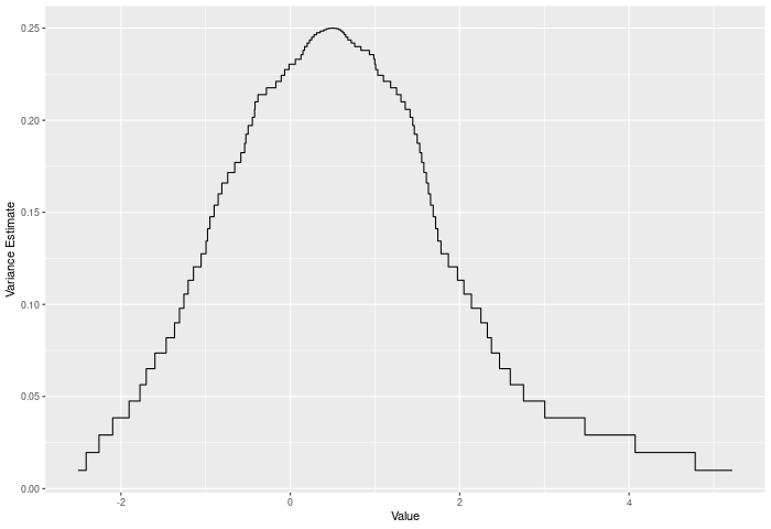
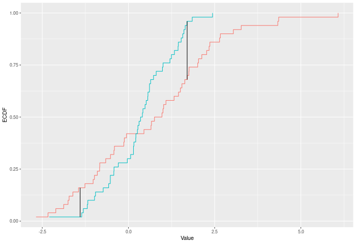
The AD test compares two ECDFs by looking at the weighted sum of the squared differences between them – evaluated at each point in the joint sample. The weights are determined by the variance of the joint ECDF at that point, which peaks in the middle of the joint distribution (see figure below). Formally – if E is the ECDF of sample 1, F is the ECDF of sample 2, and G is the ECDF of the joint sample then

AD = \sum_{x \in k} \left({|E(x)-F(x)| \over \sqrt{2G(x)(1-G(x))/n} }\right)^p

where k is the joint sample. The test p-value is calculated by randomly resampling two samples of the same size using the combined sample. Intuitively the AD test improves on the CVM test by giving lower weight to noisy observations.

In the example plot below, we see the variance of the joint ECDF over the range of the data. It clearly peaks in the middle of the joint sample.

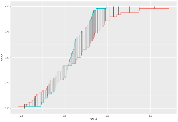
In the example plot below, the AD statistic is the weighted sum of the heights of the vertical lines, where weights are represented by the shading of the lines.

Inputs a and b can also be vectors of ordered (or unordered) factors, so long as both have the same levels and orderings. When possible, ordering factors will substantially increase power.

Value

Output is a length 2 Vector with test stat and p-value in that order. That vector has 3 attributes – the sample sizes of each sample, and the number of bootstraps performed for the pvalue.

Functions

• ad_test(): Permutation based two sample Anderson-Darling test

• ad_stat(): Permutation based two sample Anderson-Darling test

See Also

dts_test() for a more powerful test statistic. See cvm_test() for the predecessor to this test statistic. See dts_test() for the natural successor to this test statistic.

Examples

set.seed(314159)
vec1 = rnorm(20)
vec2 = rnorm(20,0.5)
out = ad_test(vec1,vec2)
out
summary(out)
plot(out)

# Example using ordered factors
vec1 = factor(LETTERS[1:5],levels = LETTERS,ordered = TRUE)
vec2 = factor(LETTERS[c(1,2,2,2,4)],levels = LETTERS, ordered=TRUE)
ad_test(vec1,vec2)

Combine two objects of class twosamples

Description

This function combines two twosamples objects – concatenating bootstraps, recalculating pvalues, etc. It only works if both objects were created with "keep.boots=T" This function is intended for one main purposes: combining parallized null calculations and then plotting those combined outputs.

Usage

combine.twosamples(x, y, check.sample = T)

Arguments

Value

a twosamples object that correctly re-calculates the p-value and determines all the other attributes

See Also

twosamples_class, plot.twosamples, dts_test

Examples

vec1 = rnorm(10)
vec2 = rnorm(10,1)
out1 = dts_test(vec1,vec2)
out2 = dts_test(vec1,vec2)
combined = combine.twosamples(out1,out2)
summary(out1)
summary(out2)
summary(combined)
plot(combined)

Cramer-von Mises Test

Description

A two-sample test based on the Cramer-Von Mises test statistic (cvm_stat).

Usage

cvm_test(a, b, nboots = 2000, p = default.p, keep.boots = T, keep.samples = F)

cvm_stat(a, b, power = def_power)

Arguments

Details

The CVM test compares two ECDFs by looking at the sum of the squared differences between them – evaluated at each point in the joint sample. Formally – if E is the ECDF of sample 1 and F is the ECDF of sample 2, then

CVM = \sum_{x\in k}|E(x)-F(x)|^p

where k is the joint sample. The test p-value is calculated by randomly resampling two samples of the same size using the combined sample. Intuitively the CVM test improves on KS by using the full joint sample, rather than just the maximum distance – this gives it greater power against shifts in higher moments, like variance changes.

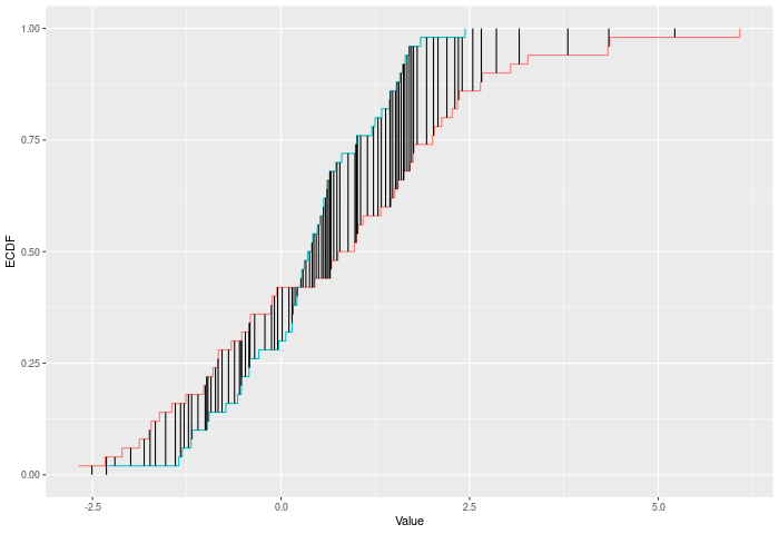
In the example plot below, the CVM statistic is the sum of the heights of the vertical black lines.

Inputs a and b can also be vectors of ordered (or unordered) factors, so long as both have the same levels and orderings. When possible, ordering factors will substantially increase power.

Value

Output is a length 2 Vector with test stat and p-value in that order. That vector has 3 attributes – the sample sizes of each sample, and the number of bootstraps performed for the pvalue.

Functions

• cvm_test(): Permutation based two sample Cramer-Von Mises test

• cvm_stat(): Permutation based two sample Cramer-Von Mises test

See Also

dts_test() for a more powerful test statistic. See ks_test() or kuiper_test() for the predecessors to this test statistic. See wass_test() and ad_test() for the successors to this test statistic.

Examples

set.seed(314159)
vec1 = rnorm(20)
vec2 = rnorm(20,0.5)
out = cvm_test(vec1,vec2)
out
summary(out)
plot(out)

# Example using ordered factors
vec1 = factor(LETTERS[1:5],levels = LETTERS,ordered = TRUE)
vec2 = factor(LETTERS[c(1,2,2,2,4)],levels = LETTERS, ordered=TRUE)
cvm_test(vec1,vec2)

Kolmogorov-Smirnov Test

Description

A two-sample test using the Kolmogorov-Smirnov test statistic (ks_stat).

Usage

ks_test(a, b, nboots = 2000, p = default.p, keep.boots = T, keep.samples = F)

ks_stat(a, b, power = def_power)

Arguments

Details

The KS test compares two ECDFs by looking at the maximum difference between them. Formally – if E is the ECDF of sample 1 and F is the ECDF of sample 2, then

KS = max |E(x)-F(x)|^p

for values of x in the joint sample. The test p-value is calculated by randomly resampling two samples of the same size using the combined sample.

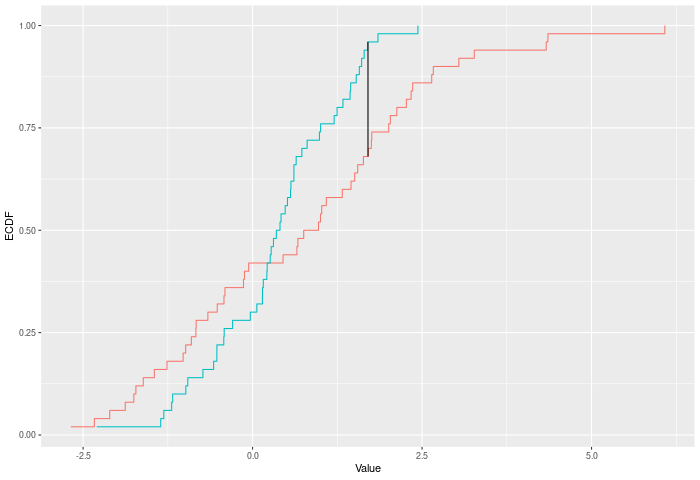
In the example plot below, the KS statistic is the height of the vertical black line.

Inputs a and b can also be vectors of ordered (or unordered) factors, so long as both have the same levels and orderings. When possible, ordering factors will substantially increase power.

Value

Output is a length 2 Vector with test stat and p-value in that order. That vector has 3 attributes – the sample sizes of each sample, and the number of bootstraps performed for the pvalue.

Functions

• ks_test(): Permutation based two sample Kolmogorov-Smirnov test

• ks_stat(): Permutation based two sample Kolmogorov-Smirnov test

See Also

dts_test() for a more powerful test statistic. See kuiper_test() or cvm_test() for the natural successors to this test statistic.

Examples

set.seed(314159)
vec1 = rnorm(20)
vec2 = rnorm(20,0.5)
out = ks_test(vec1,vec2)
out
summary(out)
plot(out)

# Example using ordered factors
vec1 = factor(LETTERS[1:5],levels = LETTERS,ordered = TRUE)
vec2 = factor(LETTERS[c(1,2,2,2,4)],levels = LETTERS, ordered=TRUE)
ks_test(vec1,vec2)

Kuiper Test

Description

A two-sample test based on the Kuiper test statistic (kuiper_stat).

Usage

kuiper_test(
  a,
  b,
  nboots = 2000,
  p = default.p,
  keep.boots = T,
  keep.samples = F
)

kuiper_stat(a, b, power = def_power)

Arguments

Details

The Kuiper test compares two ECDFs by looking at the maximum positive and negative difference between them. Formally – if E is the ECDF of sample 1 and F is the ECDF of sample 2, then

KUIPER = |max_x E(x)-F(x)|^p + |max_x F(x)-E(x)|^p

. The test p-value is calculated by randomly resampling two samples of the same size using the combined sample.

In the example plot below, the Kuiper statistic is the sum of the heights of the vertical black lines.

Inputs a and b can also be vectors of ordered (or unordered) factors, so long as both have the same levels and orderings. When possible, ordering factors will substantially increase power.

Value

Output is a length 2 Vector with test stat and p-value in that order. That vector has 3 attributes – the sample sizes of each sample, and the number of bootstraps performed for the pvalue.

Functions

• kuiper_test(): Permutation based two sample Kuiper test

• kuiper_stat(): Permutation based two sample Kuiper test

See Also

dts_test() for a more powerful test statistic. See ks_test() for the predecessor to this test statistic, and cvm_test() for its natural successor.

Examples

set.seed(314159)
vec1 = rnorm(20)
vec2 = rnorm(20,0.5)
out = kuiper_test(vec1,vec2)
out
summary(out)
plot(out)


# Example using ordered factors
vec1 = factor(LETTERS[1:5],levels = LETTERS,ordered = TRUE)
vec2 = factor(LETTERS[c(1,2,2,2,4)],levels = LETTERS, ordered=TRUE)
kuiper_test(vec1,vec2)

Permutation Test Builder

Description

(Warning! This function has changed substantially between v1.2.0 and v2.0.0) This function takes a two-sample test statistic and produces a function which performs randomization tests (sampling with replacement) using that test stat. This is an internal function of the twosamples package.

Usage

permutation_test_builder(test_stat_function, default.p = 2)

Arguments

Details

test_stat_function must be structured to take two vectors – the first a combined sample vector and the second a logical vector indicating which sample each value came from, as well as a third and fourth value. i.e. (fun = function(jointvec,labelvec,val1,val2) ...). See examples.

Conversion Function

Test stat functions designed to work with the prior version of permutation_test_builder will not work. E.g. If your test statistic is

mean_diff_stat = function(x,y,pow) abs(mean(x)-mean(y))^pow

then permutation_test_builder(mean_diff_stat,1) will no longer work as intended, but it will if you run the below code first.

perm_stat_helper = function(stat_fn,def_power) {
  output = function(joint,vec_labels,power=def_power,na) {
    a = joint[vec_labels]
    b = joint[!vec_labels]
    stat_fn(a,b,power)
  }
  output
}

mean_diff_stat = perm_stat_helper(mean_diff_stat)

Value

This function returns a function which will perform permutation tests on given test stat.

Functions

• permutation_test_builder(): Takes a test statistic, returns a testing function.

See Also

two_sample()

Examples

mean_stat = function(joint,label,p,na) abs(mean(joint[label])-mean(joint[!label]))**p
myfun = twosamples:::permutation_test_builder(mean_stat,2.0)
set.seed(314159)
vec1 = rnorm(20)
vec2 = rnorm(20,0.5)
out = myfun(vec1,vec2)
out
summary(out)
plot(out)

Default plots for twosamples objects

Description

Typically for now this will produce a histogram of the null distribution based on the bootstrapped values, with a vertical line marking the value of the test statistic.

Usage

## S3 method for class 'twosamples'
plot(x, plot_type = c("boots_hist"), nbins = 50, ...)

Arguments

Value

Produces a plot

See Also

dts_test(), twosamples_class, combine.twosamples

Examples

out = dts_test(rnorm(10),rnorm(10,1))
plot(out)

twosamples_class

Description

Objects of Class twosamples are output by all of the ⁠*_test⁠ functions in the twosamples package.

Usage

## S3 method for class 'twosamples'
print(x, ...)

## S3 method for class 'twosamples'
summary(object, alpha = 0.05, ...)

Arguments

Details

By default they consist of:a length 2 vector, the first item being the test statistic, the second the p-value. That vector has the following attributes:

1. details: length 3 vector with the sample sizes for each sample and the number of bootstraps

2. test_type: a string describing the type of the test statistic

It may also have two more attributes, depending on options used when running the ⁠*_test⁠ function. These are useful for plotting and combining test runs.

1. bootstraps: a vector containing all the bootstrapped null values

2. samples: a list containing both the samples that were tested

and by virtue of being a named length 2 vector of class "twosamples" it has the following two attributes:

1. names: c("Test Stat","P-Value")

2. class: "twosamples"

Multiple Twosamples objects made by the same ⁠*_test⁠ routine being run on the same data can be combined (getting correct p-value and correct attributes) with the function combine_twosamples().

Value

• print.twosamples() returns nothing

• summarize.twosamples() returns nothing

Functions

• print(twosamples): Print method for objects of class twosamples

• summary(twosamples): Summary method for objects of class twosamples

See Also

plot.twosamples(), combine.twosamples()

DTS Test

Description

A two-sample test based on the DTS test statistic (dts_stat). This is the recommended two-sample test in this package because of its power. The DTS statistic is the reweighted integral of the distance between the two ECDFs.

Usage

dts_test(a, b, nboots = 2000, p = default.p, keep.boots = T, keep.samples = F)

two_sample(
  a,
  b,
  nboots = 2000,
  p = default.p,
  keep.boots = T,
  keep.samples = F
)

dts_stat(a, b, power = def_power)

Arguments

Details

The DTS test compares two ECDFs by looking at the reweighted Wasserstein distance between the two. See the companion paper at arXiv:2007.01360 or https://codowd.com/public/DTS.pdf for details of this test statistic, and non-standard uses of the package (parallel for big N, weighted observations, one sample tests, etc).

If the wass_test() extends cvm_test() to interval data, then dts_test() extends ad_test() to interval data. Formally – if E is the ECDF of sample 1, F is the ECDF of sample 2, and G is the ECDF of the combined sample, then

DTS = \int_{x\in R} \left({|E(x)-F(x)| \over \sqrt{2G(x)(1-G(x))/n}}\right)^p

for all x. The test p-value is calculated by randomly resampling two samples of the same size using the combined sample. Intuitively the DTS test improves on the AD test by allowing more extreme observations to carry more weight. At a higher level – CVM/AD/KS/etc only require ordinal data. DTS (and Wasserstein) gain power because they take advantages of the properties of interval data – i.e. the distances have some meaning. However, DTS, like Anderson-Darling (AD) also downweights noisier observations relative to Wass, thus (hopefully) giving it extra power.

In the example plot below, the DTS statistic is the shaded area between the ECDFs, weighted by the variances – shown by the color of the shading.

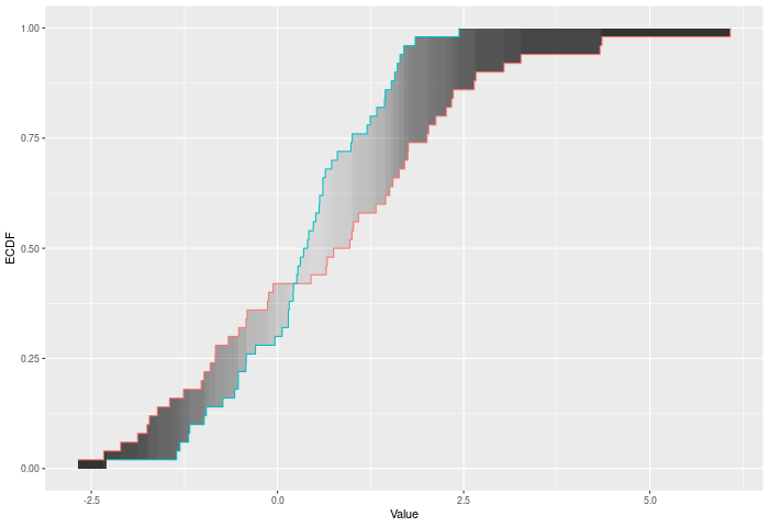
Inputs a and b can also be vectors of ordered (or unordered) factors, so long as both have the same levels and orderings. When possible, ordering factors will substantially increase power. The dts test will assume the distance between adjacent factors is 1.

Value

Output is a length 2 Vector with test stat and p-value in that order. That vector has 3 attributes – the sample sizes of each sample, and the number of bootstraps performed for the pvalue.

Functions

• dts_test(): Permutation based two sample test

• two_sample(): Recommended two-sample test

• dts_stat(): Permutation based two sample test

See Also

wass_test(), ad_test() for the predecessors of this test statistic. arXiv:2007.01360 or https://codowd.com/public/DTS.pdf for details of this test statistic

Examples

set.seed(314159)
vec1 = rnorm(20)
vec2 = rnorm(20,0.5)
dts_stat(vec1,vec2)
out = dts_test(vec1,vec2)
out
summary(out)
plot(out)
two_sample(vec1,vec2)

# Example using ordered factors
vec1 = factor(LETTERS[1:5],levels = LETTERS,ordered = TRUE)
vec2 = factor(LETTERS[c(1,2,2,2,4)],levels = LETTERS, ordered=TRUE)
dts_test(vec1,vec2)

Wasserstein Distance Test

Description

A two-sample test based on Wasserstein's distance (wass_stat).

Usage

wass_test(a, b, nboots = 2000, p = default.p, keep.boots = T, keep.samples = F)

wass_stat(a, b, power = def_power)

Arguments

Details

The Wasserstein test compares two ECDFs by looking at the Wasserstein distance between the two. This is of course the area between the two ECDFs. Formally – if E is the ECDF of sample 1 and F is the ECDF of sample 2, then

WASS = \int_{x \in R} |E(x)-F(x)|^p

across all x. The test p-value is calculated by randomly resampling two samples of the same size using the combined sample. Intuitively the Wasserstein test improves on CVM by allowing more extreme observations to carry more weight. At a higher level – CVM/AD/KS/etc only require ordinal data. Wasserstein gains its power because it takes advantages of the properties of interval data – i.e. the distances have some meaning.

In the example plot below, the Wasserstein statistic is the shaded area between the ECDFs.

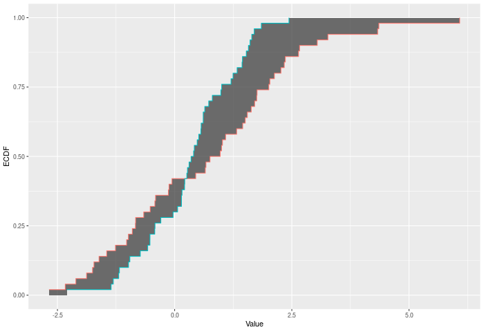
Inputs a and b can also be vectors of ordered (or unordered) factors, so long as both have the same levels and orderings. When possible, ordering factors will substantially increase power. wass_test will assume the distance between adjacent factors is 1.

Value

Output is a length 2 Vector with test stat and p-value in that order. That vector has 3 attributes – the sample sizes of each sample, and the number of bootstraps performed for the pvalue.

Functions

• wass_test(): Permutation based two sample test using Wasserstein metric

• wass_stat(): Permutation based two sample test using Wasserstein metric

See Also

dts_test() for a more powerful test statistic. See cvm_test() for the predecessor to this test statistic. See dts_test() for the natural successor of this test statistic.

Examples

set.seed(314159)
vec1 = rnorm(20)
vec2 = rnorm(20,0.5)
out = wass_test(vec1,vec2)
out
summary(out)
plot(out)

# Example using ordered factors
vec1 = factor(LETTERS[1:5],levels = LETTERS,ordered = TRUE)
vec2 = factor(LETTERS[c(1,2,2,2,4)],levels = LETTERS, ordered=TRUE)
wass_test(vec1,vec2)