| Type: | Package |
| Title: | Soil Physical Analysis |
| Version: | 5.0 |
| Date: | 2022-06-06 |
| Description: | Basic and model-based soil physical analyses. |
| Author: | Anderson Rodrigo da Silva
 [aut, cre],
Renato Paiva de Lima
[aut] [aut, cre],
Renato Paiva de Lima
[aut] |
| Maintainer: | Anderson Rodrigo da Silva <anderson.agro@hotmail.com> |
| URL: | https://arsilva87.github.io/soilphysics/ |
| Imports: | utils, stats, graphics, boot, grDevices, datasets, MASS, shiny, rhandsontable, shinydashboard, fields |
| Suggests: | knitr, rmarkdown, rpanel, tcltk |
| VignetteBuilder: | knitr |
| License: | GPL-2 | GPL-3 [expanded from: GPL (≥ 2)] |
| NeedsCompilation: | no |
| Packaged: | 2022-06-07 15:25:34 UTC; User |
| Repository: | CRAN |
| Date/Publication: | 2022-06-07 16:10:02 UTC |
Soil Physical Analysis
Description
Basic and model-based soil physical analyses.
Details
| Package: | soilphysics |
| Type: | Package |
| Version: | 5.0 |
| Date: | 2022-06-06 |
| License: | GPL (>= 2) |
Functions for modelling the load bearing capacity and the penetration resistance, and for predicting the stress applied by agricultural machines in the soil profile. The package allows one to model the soil water retention through six different models. There are some useful and easy-to-use functions to perform parameter estimation of these models. Methods to obtain the preconsolidation stress are available, such as the standard of Casagrande (1936) and so on. It is possible to quantify soil water availability for plants through the Least Limiting Water Range approach as well as the Integral Water Capacity. Moreover, it is possible to determine the water suction at the point of hydraulic cut-off. Also, users can deal with the high-energy-moisture-characteristics (HEMC) methodology proposed by Pierson and Mulla (1989), which is used to analyze the aggregate stability. There is a function to determine the soil critical moisture and the maximum bulk density for one or more samples, based on the Proctor (1933) compaction test. Other utilities like a function to calculate the soil liquid limit, the void ratio and to determine the maximum curvature point are available.
Note
soilphysics is an ongoing project. We welcome any and all criticism, comments and suggestions.
Author(s)
Anderson Rodrigo da Silva, Renato Paiva de Lima
Maintainer: Anderson Rodrigo da Silva <anderson.agro@hotmail.com>
References
da Silva, A.R.; de Lima, R.P. (2015) soilphysics: an R package to determine soil preconsolidation pressure. Computers and Geosciences, 84: 54-60.
de Lima, R.P.; da Silva, A.R.; da Silva, A.P.; Leao, T.P.; Mosaddeghi, M.R. (2016) soilphysics: an R package for calculating soil water availability to plants by different soil physical indices. Computers and Eletronics in Agriculture, 120: 63-71.
da Silva, A.R.; Lima, R.P. (2017) Determination of maximum curvature point with the R package soilphysics. International Journal of Current Research, 9: 45241-45245.
De Lima, R.P.; Da Silva, A.R.; Da Silva, A.P. (2021) soilphysics: An R package for simulation of soil compaction induced by agricultural field traffic. SOIL and TILLAGE RESEARCH, 206: 104824.
Unsaturated Hydraulic Conductivity
Description
A closed-form analytical expressions for calculating the relative unsaturated hydraulic conductivity as a function of soil water tension (h) based on van Genuchten's water retention curve.
Usage
Kr_h(Ks, alpha, n, h, f=0.5)
Arguments
Ks |
Saturated hydraulic conductivity (e.g. cm/day). |
alpha |
The scale parameter of the van Genuchten's model (hPa^-1). |
n |
The shape parameter in van Genuchten's formula. |
h |
The water tension (hPa). |
f |
The pore-connectivity parameter. Default 0.5 [Mualem, 1976]. |
Value
numeric, the value of unsaturated hydraulic conductivity.
Author(s)
Renato Paiva de Lima <renato_agro_@hotmail.com>
References
Guarracino, L. (2007). Estimation of saturated hydraulic conductivity Ks from the van Genuchten shape parameter alpha. Water Resources Research, 43(11).
Van Genuchten, M. T. (1980). A closed-form equation for predicting the hydraulic conductivity of unsaturated soils 1. Soil Science Society of America Journal 44(5):892-898.
Examples
# EXAMPLE 1
Kr_h(Ks = 1.06*10^2, alpha = 0.048, n = 1.5,h=100, f=0.5)

# EXAMPLE 2
x <- seq(log10(1), log10(1000),len=100)
h <- 10^x
y <- Kr_h(Ks = 1.06*10^2, alpha = 0.048, n = 1.5,h=h, f=0.5)
plot(x=h,y=y, log="yx", xlab="h (hPa)", yaxt='n',
    ylab="", ylim=c(0.001,100), xlim=c(1,10000))
mtext(expression(K[r] ~ (cm~d^-1)), 2, line=2)
ax <- c(0.001, 0.01, 0.1, 1, 10, 100)
axis(2,at=ax, labels=ax)

# End (not run)
Unsaturated Hydraulic Conductivity as a function of water content
Description
A closed-form analytical expressions for calculating the relative unsaturated hydraulic conductivity as a function of soil water content based on van Genuchten's water retention curve.
Usage
Kr_theta(theta, thetaS, thetaR, n, Ks, f=0.5)
Arguments
theta |
The volumetric water content (m^3/m^3). |
thetaS |
The volumetric water content at the saturation (m^3/m^3). |
thetaR |
The volumetric residual water content (m^3/m^3). |
n |
The shape parameter in van Genuchten's formula. |
Ks |
Saturated hydraulic conductivity (e.g. cm/day). |
f |
The pore-connectivity parameter. Default 0.5 [Mualem, 1976]. |
Value
numeric, the value of unsaturated hydraulic conductivity.
Author(s)
Renato Paiva de Lima <renato_agro_@hotmail.com>
References
Guarracino, L. (2007). Estimation of saturated hydraulic conductivity Ks from the van Genuchten shape parameter alpha. Water Resources Research, 43(11).
Van Genuchten, M. T. (1980). A closed-form equation for predicting the hydraulic conductivity of unsaturated soils. Soil Science Society of America Journal 44(5):892-898.
Mualem, Y. (1976). A new model for predicting the hydraulic conductivity of unsaturated porous media. Water Resour. Res. 43(11): 513-522,
Examples
# EXAMPLE 1
Kr_theta(theta=0.45,thetaS=0.5,thetaR=0.15,
         n = 2, Ks = 1.06*10^2, f=0.5)

# EXAMPLE 2
thetaS <- 0.50
thetaR <- 0.15
theta <- seq(thetaS, thetaR, len=50)
y <- Kr_theta(theta=theta,thetaS=thetaS,thetaR=thetaR,
             n = 2, Ks = 1.06*10^2, f=0.5)

# Just for this example, we are removing the "0" value
# for plotting the graph in log scale, sence log10(0) results in "-Inf"
Kr <- y[-50]
w <- theta[-50]

plot(x=w,y=Kr,xlab=expression(theta~(m^3~m^-3)),
     ylim=c(0.001,100), log="y",yaxt='n',
     ylab="", xlim=c(0.15,0.50))
mtext(expression(K[r] ~ (cm~d^-1)), 2, line=2)
ax <- c(0.001, 0.01, 0.1, 1, 10, 100)
axis(2,at=ax, labels=ax)

# End (not run)
A shiny for calculation of the usual least limiting water range
Description
A shiny for calculation of the usual least limiting water range
Usage
LLWR_App()
Value
A shiny app
Author(s)
Renato Paiva de Lima <renato_agro_@hotmail.com>
See Also
A shiny for calculation of least limiting water and matric potential ranges of agricultural soils with calculated physical restriction thresholds
Description
A shiny for calculation of least limiting water and matric potential ranges of agricultural soils with calculated physical restriction thresholds
Usage
LLWR_LLMPR_App()
Value
A shiny app
Author(s)
Renato Paiva de Lima <renato_agro_@hotmail.com>
See Also
A shiny for simulation of soil compaction
Description
A shiny for for simulation of soil compaction
Usage
PredComp()
Value
A shiny app
Author(s)
Renato Paiva de Lima <renato_agro_@hotmail.com>
See Also
Multiple R-squared
Description
Function to calculate the multiple R-squared and the adjusted
R-squared from a fitted model via lm or aov, i.e., linear models.
For a model fitted via nls, nonlinear models, the pseudo R-squared is
returned.
Usage
Rsq(model) Arguments
model |
Value
A list of
R.squared |
the multiple R-squared (for linear models) or the Pseudo R-squared (for nonlinear models). |
adj.R.squared |
the adjusted R-squared. |
Author(s)
Anderson Rodrigo da Silva <anderson.agro@hotmail.com>
See Also
lm, summary.lm, aov,
nls
Examples
# example 1 [linear model]
y <- rnorm(10)
x <- 1:10
fit <- lm(y ~ x)
summary(fit)
Rsq(fit)

# example 2 [nonlinear model for Load Bearing Capacity]
data(compaction)
attach(compaction)
out <- fitlbc(theta = Mois, sigmaP = PS)
summary(out)
Rsq(out)

# End (not run)
Self-Starting Nls Load Bearing Capacity Model
Description
A selfStart model that evaluates the Load Bearing Capacity
(Dias Jr., 1994) function and its gradient. It has an initial attribute
that creates initial estimates of the parameters b0 and b1.
Usage
SSlbc(theta, b0, b1) Arguments
theta |
a numeric vector of soil moisture values at which to evaluate the model. |
b0 |
a numeric parameter. |
b1 |
a numeric parameter. |
Value
a numeric vector with the same length of theta. It is the value of the
expression 10^{(b0 + b1 * \theta)}. Also, the gradient matrix with respect
to the parameters is attached as an attribute named gradient.
Author(s)
Anderson Rodrigo da Silva <anderson.agro@hotmail.com>
References
Dias Junior, M. S. (1994). Compression of three soils under longterm tillage and wheel traffic. 1994. 114p. Ph.D. Thesis - Michigan State University, East Lansing.
See Also
getInitiallbc, fitlbc, selfStart,
nls, sigmaP
Examples
data(compaction)
attach(compaction)
ss <- SSlbc(Mois, 2.79, -2.33)
ss[1:50] # prediction
PS # original data of preconsolidation stress
ss # prediction and gradient

# End (not run)
The S Index
Description
Function to calculate the S index (Dexter, 2004) for evaluating the soil physical quality based on the Water Retention Curve (van Genuchten, 1980).
S = - n * (\theta_S - \theta_R) * (1 + 1/m)^{-(1 + m)}
Usage
Sindex(theta_R, theta_S, alpha, n, m = 1 - 1/n, vcov = NULL,
	nsim = 999, conf.level = 0.95, graph = TRUE, ...)
Arguments
theta_R |
the residual water content. |
theta_S |
the water content at saturation. |
alpha |
a scale parameter of the van Genuchten's formula. |
n |
a shape parameter in van Genuchten's formula. |
m |
a shape parameter in van Genuchten's Formula. Default is |
vcov |
optional (default is |
nsim |
the number of Monte Carlo simulations; default is 999. It is used only if |
conf.level |
the confidence level; default is 0.95. It is used only if |
graph |
logical; if TRUE (defaul), the soil water retention curve is plotted. |
... |
further graphical arguments. |
Value
A list of
h_i |
the modulus of the water potential at the inflection point. |
theta_i |
the water content at the inflection point. |
S.index |
the modulus of the S index. |
PhysicalQuality |
A character indicating the soil physical quality, as proposed by Dexter (2004). |
simCI |
the simulated confidence interval. It is stored only if |
conf.level |
the confidence level for the simulated confidence interval. It is stored only if |
Author(s)
Anderson Rodrigo da Silva <anderson.agro@hotmail.com>
References
Dexter, A. R. (2004). Soil physical quality Part I. Theory, effects of soil texture, density, and organic matter, and effects on root growth. Geoderma, 120:201-214.
Genuchten, M. T. van. (1980). A closed form equation for predicting the hydraulic conductivity of unsaturated soils. Soil Science Society of America Journal, 44:892-898.
Mualem, Y. (1976). A new model for predicting the hydraulic conductivity of unsaturated porous media, Water Resource Research, 12:513-522.
See Also
Examples
# Dexter (2004, Table 1)
Sindex(0, 0.395, 0.0217, 1.103, xlim = c(0, 1000))
Sindex(0, 0.335, 0.0616, 1.139, xlim = c(0, 1000))
# ...
Sindex(0, 0.226, 0.0671, 1.581, xlim = c(0, 1000))

# End (not run)
Soil Aggregate Size Data Set
Description
Data set for determining soil aggregate size distribution.
Usage
data(SoilAggregate)Format
A data frame with 12 observations on 7 variables.
IDa factor with the names of the soil samples.
D3D1.5D0.75D0.375D0.178D0.053
Examples
data(SoilAggregate)
summary(SoilAggregate)
A shiny to automatically fit the water retention curve
Description
Use the maximum likelihood method to find the water retention curve that best fits the data.
Usage
WRC_App()
Value
A shiny app
Author(s)
Anderson Rodrigo da Silva <anderson.agro@hotmail.com>
See Also
Soil Aggregate-Size Distribution
Description
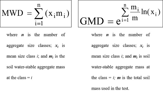
It calculates the mean weight diameter (MWD), the geometric mean diameter (GMD) and the soil aggregates size distribution per class based on the mass of the aggregates retained in each sieve from a total soil mass used for the soil aggregate stability test.
Usage
aggreg.stability(sample.id = NA, dm.classes, aggre.mass)
Arguments
sample.id |
optional; a character vector containing the sample names. |
dm.classes |
a numeric vector containing the aggregates classes, in mm. |
aggre.mass |
a |
Details
The user must arrange a data.frame with lines representing the samples and the columns representing the mass
of the aggregates retained in each one of the meshes (corresponding to each size class) in the aggregate stability test.
Value
A data.frame containing valor of MWD, GMD, total soil mass (total.mass) used in the aggregate stability
test and the percentage of soil aggregate size distribution per class.
Author(s)
Renato Paiva de Lima <renato_agro_@hotmail.com>
References
W. Kemper, W. Chepil. (1965). Size distribution of aggregates. C. Black (Ed.). Methods of Soil Analysis, American Society Agronomy, Madison. pp. 499-510.
Yoder, R. A. (1936). A direct method of aggregate analysis of soils and a study of the physical nature of erosion losses. Journal of the American Society of Agronomy, 28:337-351.
Examples
data(SoilAggregate)
classes <- c(3, 1.5, 0.75, 0.375, 0.178, 0.053)
aggreg.stability(sample.id = SoilAggregate[ ,1],
   dm.classes = classes, aggre.mass = SoilAggregate[ ,-1])

# End (not run)
A shiny for Soil Aggregate-Size Distribution
Description
A shiny for Soil Aggregate-Size Distribution
Usage
aggreg.stability_App()
Value
A shiny app
Author(s)
Renato Paiva de Lima <renato_agro_@hotmail.com>
See Also
Soil Bulk Density Data Set
Description
This data set refers to five observations of soil bulk density and soil moisture per sample. There are four soil samples.
Usage
data(bulkDensity) Format
A data frame with 20 observations on the following 3 variables.
Ida factor with levels
s1s2s3s4, the 'ID' of each soil sample.MOISa numeric vector containing soil moisture values (cm^3 / cm^3).
BULKa numeric vector containing soil bulk density values (g / cm^3).
Source
Simulated data.
Examples
data(bulkDensity)
summary(bulkDensity)
Soil Compaction Data Set
Description
This data set refers to physical soil variables related to soil compaction.
Usage
data(compaction) Format
A data frame with 50 observations on the following 4 variables.
PRa numeric vector containing soil penetration resistance values (MPa).
BDa numeric vector containing soil bulk density values (g / cm^3).
Moisa numeric vector containing soil moisture values (cm^3 / cm^3).
PSa numeric vector containing soil preconsolidation stress values (kPa).
Source
Simulated data.
Examples
data(compaction)
summary(compaction)
Estimation of compressive properties by Defossez et al. (2003)
Description
It calculates the compressive parameters N and lambda using the pedo-transfer function from Defossez et al. (2003)
Usage
compressive_properties(water.content, soil=c("Loess", "Calcareous"))
Arguments
water.content |
a numeric vector containing the values of gravimetric water content, |
soil |
the soil group 'Loess' or 'Calcareous'. See examples |
Details
In Defossez et al. (2003), the recompression index, kappa, was assumed as 0.0058 for both soil group.
Value
N |
the specific volume at |
CI |
the compression index, lambda |
Author(s)
Renato Paiva de Lima <renato_agro_@hotmail.com> Anderson Rodrigo da Silva <anderson.agro@hotmail.com>
References
Defossez, P., Richard, G., Boizard, H., & O'Sullivan, M. F., 2003. Modeling change in soil compaction due to agricultural traffic as function of soil water content. Geoderma, 116: 89–105.
See Also
Examples
# EXAMPLE 1 - For Loess and Calcareous soil

water.content <- 25
compressive_properties(water.content=water.content, soil="Loess")
compressive_properties(water.content=water.content, soil="Calcareous")

# EXAMPLE 2 - For Loess soil

water.content <- seq(from=5,to=30,len=20)
out <- compressive_properties(water.content=water.content, soil="Loess")
plot(x=water.content ,y=out$N, ylab="N", xlab="Bulk density") # plot for N
plot(x=water.content ,y=out$CI, ylab="Lambda", xlab="Bulk density") # plot for compression index


# EXAMPLE 3 - For Calcareous soil

water.content <- seq(from=5,to=30,len=20)
out <- compressive_properties(water.content=water.content, soil="Calcareous")
plot(x=water.content ,y=out$N, ylab="N", xlab="Bulk density") # plot for N
plot(x=water.content ,y=out$CI, ylab="Lambda", xlab="Bulk density") # plot for compression index

# End (not run)
Estimation of compressive properties by Keller and Arvidsson (2007)
Description
It calculates the compressive parameters N and lambda using the pedo-transfer function from Keller and Arvidsson (2007)
Usage
compressive_properties2(particle.density, bulk.density)
Arguments
particle.density |
a numeric vector containing the values of particle density, |
bulk.density |
a numeric vector containing the values of bulk density, |
Details
In Keller and Arvidsson (2007), the recompression index, kappa, was found as 0.042 for all soil.
Value
N |
the specific volume at |
CI |
the compression index, lambda |
Author(s)
Renato Paiva de Lima <renato_agro_@hotmail.com> Anderson Rodrigo da Silva <anderson.agro@hotmail.com>
References
Keller, T., Arvidsson, J., 2007. Compressive properties of some Swedish and Danish structured agricultural soils measured in uniaxial compression tests. European Journal of Soil Science , 58: 1373-1381.
See Also
Examples
# EXAMPLE 1

 compressive_properties2(particle.density=2.65, bulk.density=1.5)

# EXAMPLE 2

BD <- seq(from=1.2,to=1.8, by=0.01) # range of bulk density from 1.2 to 1.8
out <- compressive_properties2(particle.density=2.65, bulk.density=BD)

plot(x=BD,y=out$N, ylab="N", xlab="Bulk density") # for N
plot(x=BD,y=out$CI, ylab="Compression index (CI)", xlab="Bulk density") # for compression index

# End (not run)
Estimation of compressive properties by de Lima et al. (2018)
Description
It calculates the compressive parameters N, lambda and kappa using the pedo-transfer function from de Lima et al. (2018)
Usage
compressive_properties3(bulk.density, matric.suction, soil=c("SandyLoam","SandyClayLoam"))
Arguments
bulk.density |
a numeric vector containing the values of bulk density, |
matric.suction |
a numeric vector containing the values of matric suction, hPa |
soil |
the soil texture group 'SandyLoam' or 'SandyClayLoam'. See exemples |
Details
Pedo-transfer function deveploed under no-till condition. See de Lima et al. (2018)
Value
N |
the specific volume at |
CI |
the compression index, lambda |
k |
the recompression index, kappa |
Author(s)
Renato Paiva de Lima <renato_agro_@hotmail.com> Anderson Rodrigo da Silva <anderson.agro@hotmail.com>
References
de Lima, R. P., da Silva, A. P., Giarola, N. F., da Silva, A. R., Rolim, M. M., Keller, T., 2018. Impact of initial bulk density and matric suction on compressive properties of two Oxisols under no-till. Soil and Tillage Research, 175: 168-177.
See Also
Examples
# EXAMPLE 1

compressive_properties3(bulk.density=1.5, matric.suction=100, soil="SandyLoam")
compressive_properties3(bulk.density=1.5, matric.suction=100, soil="SandyClayLoam")

# EXAMPLE 2 for SandyLoam soil

matric.suction <- seq(from=30,to=1000,len=100)
out <- compressive_properties3(bulk.density=1.5,
	matric.suction=matric.suction, soil="SandyLoam")
plot(x=matric.suction,y=out$N, ylab="N",
	xlab="Matric suction (hPa)", log="x") # plot for N
# plot for lambda
plot(x=matric.suction,y=out$lambda, ylab="lambda",
	xlab="Matric suction (hPa)", log="x")
# plot for kappa
plot(x=matric.suction,y=out$k, ylab="kappa",
	xlab="Matric suction (hPa)", log="x")


# EXAMPLE 3 for SandyClayLoam soil

matric.suction <- seq(from=30,to=1000,len=100)
out <- compressive_properties3(bulk.density=1.5,
				matric.suction=matric.suction,
				soil="SandyClayLoam")
plot(x=matric.suction,y=out$N, ylab="N",
     xlab="Matric suction (hPa)", log="x") # plot for N
# plot for lambda
plot(x=matric.suction,y=out$lambda,
     ylab="lambda", xlab="Matric suction (hPa)", log="x")
# plot for kappa
plot(x=matric.suction,y=out$k,
     ylab="kappa", xlab="Matric suction (hPa)", log="x")

# End (not run)
Estimation of compressive properties by de Lima et al. (2020)
Description
It calculates the compressive parameters N, lambda and kappa using the pedo-transfer function from de Lima et al. (2020)
Usage
compressive_properties4(matric.suction, soil=c("PloughLayer","PloughPan"))
Arguments
matric.suction |
a numeric vector containing the values of matric suction, hPa. |
soil |
the soil compaction state 'PloughLayer' or 'PloughPan'. See the examples. |
Details
Pedo-transfer function developed for a sandy loam soil texture. See de Lima et al. (2018)
Value
N |
the specific volume at |
CI |
the compression index, lambda |
k |
the recompression index, kappa |
Author(s)
Renato Paiva de Lima <renato_agro_@hotmail.com> Anderson Rodrigo da Silva <anderson.agro@hotmail.com>
References
de Lima, R. P., Rolim, M. M., da C. Dantas, D., da Silva, A. R., Mendonca, E. A., 2020. Compressive properties and least limiting water range of plough layer and plough pan in sugarcane fields. Soil Use and Management, 00: 1-12.
See Also
Examples
# EXAMPLE 1

compressive_properties4(matric.suction=100, soil="PloughLayer")
compressive_properties4(matric.suction=100, soil="PloughPan")


# EXAMPLE 2 for "PloughLayer"

matric.suction <- seq(from=10,to=10000,len=100)
out <- compressive_properties4(matric.suction=matric.suction, soil="PloughLayer")
plot(x=matric.suction,y=out$N, ylab="N",
	xlab="Matric suction (hPa)", log="x") # plot for N
# plot for lambda
plot(x=matric.suction,y=out$lambda, ylab="lambda",
	xlab="Matric suction (hPa)", log="x")
# plot for kappa
plot(x=matric.suction,y=out$k, ylab="kappa",
	xlab="Matric suction (hPa)", log="x")


# EXAMPLE 3 for "PloughPan"

matric.suction <- seq(from=10,to=10000,len=100)
out <- compressive_properties4(matric.suction=matric.suction,
                               soil="PloughPan")
# plot for N
plot(x=matric.suction,y=out$N,
     ylab="N", xlab="Matric suction (hPa)", log="x")
# plot for lambda
plot(x=matric.suction,y=out$lambda,
     ylab="lambda", xlab="Matric suction (hPa)", log="x")
# plot for kappa
plot(x=matric.suction,y=out$k, ylab="kappa",
     xlab="Matric suction (hPa)", log="x")

# End (not run)
Estimation of compressive properties by O'Sullivan et al. (1999)
Description
It calculates the compressive parameteres N, lambda and kappa using the pedo-transfer function from O'Sullivan et al. (1999)
Usage
compressive_properties5(water.content, soil=c("SandyLoam","ClayLoam"))
Arguments
water.content |
a numeric vector containing the values of gravimetric water content, |
soil |
the the soil texture group 'SandyLoam' or 'ClayLoam'. See exemples. |
Details
See O'Sullivan et al. (1999).
Value
N |
the specific volume at |
CI |
the compression index, lambda |
k |
the recompression index, kappa |
Author(s)
Renato Paiva de Lima <renato_agro_@hotmail.com> Anderson Rodrigo da Silva <anderson.agro@hotmail.com>
References
O'sullivan, M. F., Henshall, J. K., Dickson, J. W., 1999. A simplified method for estimating soil compaction. Soil and Tillage Research, 49: 325-335.
See Also
Examples
# EXAMPLE 1
water.content <- 15
compressive_properties5(water.content=water.content, soil="SandyLoam")
compressive_properties5(water.content=water.content, soil="ClayLoam")


# EXAMPLE 2 - SandyLoam

water.content <- seq(from=5,to=20,len=20)
out <- compressive_properties5(water.content=water.content, soil="SandyLoam")
plot(x=water.content ,y=out$N,
     ylab="N", xlab="Bulk density") # plot for N
plot(x=water.content ,y=out$lambda,
    ylab="lambda", xlab="Bulk density") # plot for lambda
plot(x=water.content ,y=out$kappa,
    ylab="kappa", xlab="Bulk density") # plot for kappa


# EXAMPLE 3 - ClayLoam

water.content <- seq(from=10,to=25,len=20)
out <- compressive_properties5(water.content=water.content, soil="ClayLoam")
plot(x=water.content ,y=out$N,
     ylab="N", xlab="Bulk density") # plot for N
plot(x=water.content ,y=out$lambda,
     ylab="lambda", xlab="Bulk density") # plot for lambda
plot(x=water.content ,y=out$kappa,
     ylab="kappa", xlab="Bulk density") # plot for rkappa

# End (not run)
Critical Moisture and Maximum Bulk Density
Description
Function to determine the soil Critical Moisture and the Maximum Bulk Density based on the Proctor (1933) compaction test. It estimates compaction curve by fitting a quadradtic regression model.
Usage
criticalmoisture(theta, Bd, samples = NULL, graph = TRUE, ...)

maxbulkdensity(theta, Bd, samples = NULL, graph = TRUE, ...)
Arguments
theta |
a vector containing the soil moisture values. |
Bd |
a vector containing the the soil bulk density values. |
samples |
optional; a vector indicating the multiple samples. Default is NULL (one sample). See details. |
graph |
logical; if TRUE (default), the soil compaction curve is plotted. |
... |
further graphical arguments. |
Details
If samples is ispecified, then it must has the same length of theta and Bd.
Value
An object of class 'criticalmoisture', i.e., a matrix containing the quadratic model coefficients (rows 1 to 3), the R-squared (row 4), the sample size (row 5), the critical soil moisture (row 6) and the maximum bulk density (row 7), per sample.
Note
maxbulkdensity is just an alias of criticalmoisture.
Author(s)
Anderson Rodrigo da Silva <anderson.agro@hotmail.com>
References
Proctor, E. R. (1933). Design and construction of rolled earth dams. Eng. News Record, 3: 245-284, 286-289, 348-351, 372-376.
Silva, A. P. et al. (2010). Indicadores da qualidade fisica do solo. In: Jong Van Lier, Q. (Ed). Fisica do solo. Vicosa (MG): Sociedade Brasileira de Ciencia do Solo. p.541-281.
See Also
Examples
# example 1 (1 sample)
mois <- c(0.083, 0.092, 0.108, 0.126, 0.135)
bulk <- c(1.86, 1.92, 1.95, 1.90, 1.87)
criticalmoisture(theta = mois, Bd = bulk)

# example 2 (4 samples)
data(bulkDensity)
attach(bulkDensity)
criticalmoisture(theta = MOIS, Bd = BULK, samples = Id)

# End (not run)
Self-starting Nls Busscher's (1990) Model for Soil Penetration Resistance
Description
Function to self start the nonlinear Busscher's (1990) model for penetration
resistance, i.e., Pr = b0 * (\theta ^ {b1}) * (Bd ^ {b2}). It creates initial
estimates (by log-linearization) of the parameters b0, b1 and b2 and uses them
to provide its least-squares estimates through nls.
Usage
fitbusscher(Pr, theta, Bd, ...) Arguments
Pr |
a numeric vector containing penetration resistance values. |
theta |
a numeric vector containing soil moisture values at which to evaluate the model. |
Bd |
a numeric vector containing bulk density values at which to evaluate the model. |
... |
further arguments to |
Value
A nls output (see help(nls)).
Author(s)
Anderson Rodrigo da Silva <anderson.agro@hotmail.com>
References
Busscher, W. J. (1990). Adjustment of flat-tipped penetrometer resistance data to common water content. Transactions of the ASAE, 3:519-524.
See Also
fitlbc, nls, summary.nls,
predict.nls, Rsq
Examples
data(compaction)
attach(compaction)
out <- fitbusscher(Pr = PR, theta = Mois, Bd = BD)
summary(out)
Rsq(out)

# 3D plot
X <- seq(min(Mois), max(Mois), len = 30) # theta
Y <- seq(min(BD), max(BD), len = 30) # Bd
f <- function(x, y) coef(out)[1] * (x^coef(out)[2]) * (y^coef(out)[3])
Z <- outer(X, Y, f)
persp(X, Y, Z,
	xlab = "Soil moisture",
	ylab = "Soil bulk density",
	zlab = "Penetration resistance",
	ticktype = "detailed",
	phi = 20, theta = 30)

# End (not run)
Parameter Estimation of the Load Bearing Capacity Model
Description
This function creates initial parameter estimates of the nonlinear Load
Bearing Capacity (Dias Jr., 1994) model, i.e., \sigma_P = 10 ^ {(b0 + b1 * \theta)},
by using two methods: a getInitial method or a log-linearization. Then,
it uses them to provide its least-squares estimates via nls.
Usage
fitlbc(theta, sigmaP, ...) Arguments
theta |
a numeric vector containing soil moisture values. |
sigmaP |
a numeric vector containing values of soil preconsolidation stress. |
... |
further arguments to |
Value
A nls object.
Author(s)
Anderson Rodrigo da Silva <anderson.agro@hotmail.com>
References
Dias Junior, M. S. (1994). Compression of three soils under longterm tillage and wheel traffic. 1994. 114p. Ph.D. Thesis - Michigan State University, East Lansing.
See Also
sigmaP, fitbusscher,
maxcurv, Rsq
Examples
data(compaction)
attach(compaction)
out <- fitlbc(theta = Mois, sigmaP = PS)
summary(out)
Rsq(out)
curve(10^(coef(out)[1] + coef(out)[2]*x))

# End (not run)
Interactive Estimation of van Genuchten's (1980) Model Parameters
Description
An interactive graphical adjustment of the soil water retention curve via van Genuchten's (1980) formula. The nonlinear least-squares estimates can be achieved taking the graphical initial values.
Usage
fitsoilwater(theta, x, xlab = NULL, ylab = NULL, ...)
Arguments
theta |
a numeric vector containing the values of soil water content. |
x |
a numeric vector containing the matric potential values. |
xlab |
a label for the x axis; if is NULL, the label "Matric potential" is used. |
ylab |
a label for the y axis; if is NULL, the label "Soil water content" is used. |
... |
further graphical arguments; see |
Value
A plot of theta versus x and the curve of the current fitted model
according to the adjusted parameters in an external interactive panel.
Pressing the button "NLS estimates" a nls summary of the
fitted model is printed on console whether convergence is achieved, otherwise
a warning box of "No convergence" is shown.
Author(s)
Anderson Rodrigo da Silva <anderson.agro@hotmail.com>
References
Genuchten, M. T. van. (1980). A closed form equation for predicting the hydraulic conductivity of unsaturated soils. Soil Science Society of America Journal, 44:892-898.
See Also
Examples
# Liu et al. (2011)
h <- c(0.001, 50.65, 293.77, 790.14, 992.74, 5065, 10130, 15195)
w <- c(0.5650, 0.4013, 0.2502, 0.2324, 0.2307, 0.1926, 0.1812, 0.1730)
fitsoilwater(w, h)

# End (not run)
Interactive Estimation of the Groenevelt and Grant (2004) Model Parameters
Description
An interactive graphical adjustment of the soil water retention curve via Groenevelt and Grant (2004) formula. The nonlinear least-squares estimates can be achieved taking the graphical initial values.
Usage
fitsoilwater2(theta, x, x0 = 6.653, xlab = NULL, ylab = NULL, ...)
Arguments
theta |
a numeric vector containing the values of soil water content. |
x |
a numeric vector containing pF (pore water suction) values. See |
x0 |
the value of pF at which the soil water content becomes zero. The default is 6.653. |
xlab |
a label for the x axis; if is NULL, the label "pF" is used. |
ylab |
a label for the y axis; if is NULL, the label "Soil water content" is used. |
... |
further graphical arguments; see |
Value
A plot of theta versus x and the curve of the current fitted model
according to the adjusted parameters in an external interactive panel.
Pressing the button "NLS estimates" a nls summary of the
fitted model is printed on console whether convergence is achieved, otherwise
a warning box of "No convergence" is shown.
Author(s)
Anderson Rodrigo da Silva <anderson.agro@hotmail.com>
References
Groenevelt & Grant (2004). A newmodel for the soil-water retention curve that solves the problem of residualwater contents. European Journal of Soil Science, 55:479-485.
See Also
Examples
w <- c(0.417, 0.354, 0.117, 0.048, 0.029, 0.017, 0.007, 0)
pF <- 0:7
fitsoilwater2(w, pF)

# End (not run)
Interactive Estimation of the Dexter's (2008) Model Parameters
Description
An interactive graphical adjustment of the soil water retention curve through the Dexter's (2008) formula. The nonlinear least-squares estimates can be achieved taking the graphical initial values.
Usage
fitsoilwater3(theta, x, xlab = NULL, ylab = NULL, ...)
Arguments
theta |
a numeric vector containing the values of soil water content. |
x |
a numeric vector containing the values of applied air pressure. |
xlab |
a label for the x axis; if is NULL, the label "pF" is used. |
ylab |
a label for the y axis; if is NULL, the label "Soil water content" is used. |
... |
further graphical arguments; see |
Value
A plot of theta versus x and the curve of the current fitted model
according to the adjusted parameters in an external interactive panel.
Pressing the button "NLS estimates" a nls summary of the
fitted model is printed on console whether convergence is achieved, otherwise
a warning box of "No convergence" is shown.
Author(s)
Anderson Rodrigo da Silva <anderson.agro@hotmail.com>
References
Dexter et al. (2008). A user-friendly water retention function that takes account of the textural and structural pore spaces in soil. Geoderma, 143:243–253.
See Also
soilwater3, nls, fitsoilwater2
Examples
# data extracted from Liu et al. (2011)
h <- c(0.001, 50.65, 293.77, 790.14, 992.74, 5065, 10130, 15195)
w <- c(0.5650, 0.4013, 0.2502, 0.2324, 0.2307, 0.1926, 0.1812, 0.1730)
fitsoilwater3(w, h)

# End (not run)
Self-starting Nls Power Models for Soil Water Retention
Description
Function to self start the following nonlinear power models for soil water retention:
\theta = \exp(a + b*Bd) \psi^c
(Silva et al., 1994)
\theta = a \psi^c
(Ross et al., 1991)
where \theta is the soil water content.
fitsoilwater() creates initial estimates (by log-linearization) of the parameters a, b and c and uses them
to provide its least-squares estimates through nls.
Usage
fitsoilwater4(theta, psi, Bd, model = c("Silva", "Ross"))
Arguments
theta |
a numeric vector containing values of soil water content. |
psi |
a numeric vector containing values of water potential (Psi). |
Bd |
a numeric vector containing values of dry bulk density. |
model |
a character; the model to be used for calculating the soil water content. It must be one of the
two: |
Value
A "nls" object containing the fitted model.
Author(s)
Anderson Rodrigo da Silva <anderson.agro@hotmail.com>
References
Ross et al. (1991). Equation for extending water-retention curves to dryness. Soil Science Society of America Journal, 55:923-927.
Silva et al. (1994). Characterization of the least limiting water range of soils. Soil Science Society of America Journal, 58:1775-1781.
See Also
fitsoilwater4, soilwater, soilwater2, soilwater3
Examples
data(skp1994)
# Example 1
ex1 <- with(skp1994,
    fitsoilwater4(theta = W, psi = h, model = "Ross"))
ex1
summary(ex1)

# Example 2
ex2 <- with(skp1994,
    fitsoilwater4(theta = W, psi = h, Bd = BD, model = "Silva"))
ex2
summary(ex2)

# Not run
Interactive Estimation of the Modified van Genuchten's Model Parameters
Description
An interactive graphical adjustment of the soil water retention curve via the van Genuchten's formula, modified by Pierson and Mulla (1989). The nonlinear least-squares estimates can be achieved taking the graphical initial values. It may be useful to estimate the parameters needed in the high-energy-moisture-characteristics (HEMC) method, which is used to analyze the aggregate stability.
Usage
fitsoilwater5(theta, x, theta_S, xlab = NULL, ylab = NULL, ...)
Arguments
theta |
a numeric vector containing the values of soil water content. |
x |
a numeric vector containing the matric potential values. |
theta_S |
an offset; a value for the parameter |
xlab |
a label for the x axis; if is NULL, the label "Matric potential" is used. |
ylab |
a label for the y axis; if is NULL, the label "Soil water content" is used. |
... |
further graphical arguments; see |
Details
The parameter theta_S must be passed as an argument. It is recommended to consider it as the highest water content value in the data set or the water content at saturation.
Value
A plot of theta versus x and the curve of the current fitted model
according to the adjusted parameters in an external interactive panel.
Pressing the button "NLS estimates" a nls summary of the
fitted model is printed on console whether convergence is achieved, otherwise
a warning box of "No convergence" is shown.
Author(s)
Anderson Rodrigo da Silva <anderson.agro@hotmail.com>
References
Pierson, F.B.; Mulla, D.J. (1989) An Improved Method for Measuring Aggregate Stability of a Weakly Aggregated Loessial Soil. Soil Sci. Soc. Am. J., 53:1825–1831.
See Also
Examples
h <- seq(0.1, 40, by = 2)
w <- c(0.735, 0.668, 0.635, 0.612, 0.559, 0.462, 0.369, 0.319, 0.296, 0.282,
	0.269, 0.256, 0.249, 0.246, 0.239, 0.236, 0.229, 0.229, 0.226, 0.222)
plot(w ~ h)

# suggestions of starting values: thetaR = 0.35, alpha = 0.1, n = 10,
# b0 = 0.02, b1 = -0.0057, b2 = 0.00004 (Not run)

fitsoilwater5(theta = w, x = h, theta_S = 0.70)

# End (Not run)
A shiny for fitting soil water retention curves
Description
A shiny for fitting soil water retention curves
Usage
fitsoilwater_App()
Value
A shiny app
Author(s)
Renato Paiva de Lima <renato_agro_@hotmail.com>
See Also
Converting Function to Formula
Description
An accessorial function to convert an object of class 'function' to an object
of class 'formula'.
Usage
fun2form(fun, y = NULL) Arguments
fun |
a object of class 'function'. It must be a one-line-written function, with no curly braces "{}". |
y |
optional; a character defining the lef side of the formula, |
Value
An object of class formula.
Warning
Numerical values into fun with three or more digits may cause miscalculation.
Author(s)
Anderson Rodrigo da Silva <anderson.agro@hotmail.com>
See Also
Examples
g <- function(x) Asym * exp(-b2 * b3 ^ x) # Gompertz Growth Model
fun2form(g, "y")

# f1 <- function(w) {exp(w)} # error
# fun2form(f1, "x")
f2 <- function(w) exp(w) # ok
fun2form(f2, "x")

# End (not run)
Get Initial Parameter Estimates for the Load Bearing Capacity Model
Description
This is a getInitial function that evaluates initial parameter estimates
for the Load Bearing Capacity model via SSlbc.
Usage
getInitiallbc(theta, sigmaP) Arguments
theta |
a numeric vector containing values of soil moisture. |
sigmaP |
a numeric vector containing values of preconsolidation stress. |
Value
A numeric vector containing the estimates of the parameters b0 and b1.
Author(s)
Anderson Rodrigo da Silva <anderson.agro@hotmail.com>
References
Dias Junior, M. S. (1994). Compression of three soils under longterm tillage and wheel traffic. 1994. 114p. Ph.D. Thesis - Michigan State University, East Lansing.
See Also
getInitial, SSlbc, nls, sigmaP
Examples
data(compaction)
attach(compaction)
getInitiallbc(theta = Mois, sigmaP = PS)

# End (not run)
High-Energy-Moisture-Characteristics Aggregate Stability
Description
A function to determine the modal suction, volume of drainable pores, structural index and stability ratio
using the high-energy-moisture-characteristics (HEMC) method by Pierson & Mulla (1989), which is used to analyze
the aggregate stability. Before using hemc(), the user may estimate the parameters of the Modified van
Genuchten's Model through the function fitsoilwater5().
Usage
hemc(x, theta_R, theta_S, alpha, n, b1, b2,
	graph = TRUE, from = 1, to = 30,
	xlab = expression(Psi ~ (J~kg^{-1})),
	ylab = expression(d ~ theta/d ~ Psi), ...)
Arguments
x |
a vector containing matric potential values. |
theta_R |
a numeric vector of length two containing the parameter values in the following orde: fast and slow. |
theta_S |
a numeric vector of length two containing the parameter values in the following orde: fast and slow. |
alpha |
a numeric vector of length two containing the parameter values in the following orde: fast and slow. |
n |
a numeric vector of length two containing the parameter values in the following orde: fast and slow. |
b1 |
a numeric vector of length two containing the parameter values in the following orde: fast and slow. |
b2 |
a numeric vector of length two containing the parameter values in the following orde: fast and slow. |
graph |
logical; if TRUE (default), a graphical solution is shown). |
from |
the lower limit for the x-axis |
to |
the lower limit for the x-axis |
xlab |
a label for the x-axis |
ylab |
a label for the y-axis |
... |
further graphical arguments |
Value
A list of a two objects: 1) a matrix containing the Modal Suction, the Volume od Drainable Pores (VDP) and the Structural Index for both, fast and slow wetting; and 2) the value of Stability Ratio.
Author(s)
Anderson Rodrigo da Silva <anderson.agro@hotmail.com>
References
Pierson, F.B.; Mulla, D.J. (1989). An Improved Method for Measuring Aggregate Stability of a Weakly Aggregated Loessial Soil. Soil Sci. Soc. Am. J., 53:1825–1831.
See Also
Examples
hemc(x = seq(1, 30), theta_R = c(0.27, 0.4), theta_S = c(0.65, 0.47),
	alpha = c(0.1393, 0.0954), n = c(6.37, 7.47),
	b1 = c(-0.008421, -0.011970), b2 = c(0.0001322, 0.0001552))

# End (Not run)
The matric potential at the point of hydraulic cut-off obtained from DE (Dexter et al., 2008) and GG (Groenevelt & Grant, 2004) water retention curves.
Description
The pore water suction at the point of hydraulic cut-off occurs at the point where the residual water content, obtained from Dexter et al. (2008), intercepts with the Groenevelt & Grant (2004) retention curve.
Usage
hydraulicCutOff(theta_R, k0, k1, n, x0 = 6.653)
Arguments
theta_R |
a parameter that represents the residual water content at the the Dexter's (2008) Water Retention Model. |
k0 |
a parameter value, extracted from the water retention curve based on the Groenevelt & Grant (2004) formula. |
k1 |
a parameter value, extracted from the water retention curve based on the Groenevelt & Grant (2004) formula. |
n |
a parameter value, extracted from the water retention curve based on the Groenevelt & Grant (2004) formula. |
x0 |
the value of pF (pore water suction) at which the soil water content becomes zero. The default is 6.653. |
Value
The water suction at the point of hydraulic cut-off.
Author(s)
Anderson Rodrigo da Silva <anderson.agro@hotmail.com>
References
Dexter, A.R.; Czyz, E.A.; Richard, G.; Reszkowska, A. (2008). A user-friendly water retention function that takes account of the textural and structural pore spaces in soil. Geoderma, 143:243–253.
Groenevelt, P.H.; Grnat, C.D. (2004). A new model for the soil-water retention curve that solves the problem of residual water contents. European Journal of Soil Science, 55:479–485.
See Also
Examples
# Dexter et al. (2012), Table 4A
hydraulicCutOff(0.1130, 6.877, 0.6508, 1.0453)
hydraulicCutOff(0.1122, 12.048, 0.4338, 2.0658)

# End (not run)
The matric potential at the point of hydraulic cut-off using the point of maximum curvature of DE (Dexter et al. 2008) water retention curve.
Description
The pore water suction at the point of hydraulic cut-off occurs at the point where the residual water content, obtained from Dexter et al. (2008), intercepts with the Groenevelt & Grant (2004) retention curve. This function calculates the Hydraulic Cut-Off using the point of maximum curvature of the DE (Dexter et al. 2008) curve.
Usage
hydraulicCutOff2(theta_R, a1, a2, p1, p2, graph = FALSE, ...)
Arguments
theta_R |
the residual water content from Dexter's (2008) water retention curve (g/g). |
a1 |
a water content parameter from Dexter's (2008) water retention curve (g/g). |
a2 |
a water content parameter from Dexter's (2008) water retention curve (g/g). |
p1 |
a matric potential parameter from Dexter's (2008) water retention curve (hPa). |
p2 |
a matric potential parameter from Dexter's (2008) water retention curve (hPa). |
graph |
logical; if TRUE a graphical solution with the maximum curvature point is displayed. |
... |
further graphical arguments. See |
Details
The arguments are the fitting parameters from Dexter's (2008) water retention curve, which can be fitted using
fitsoilwater3. Further examples of how to use these parameters are given in Dexter et al. (2012).
Value
A data.frame containing the values of matric potential (hPa), pF and water content (w) at the hydraulic cut-off (hco) point.
Author(s)
Renato Paiva de Lima <renato_agro_@hotmail.com>
References
Dexter, A.R.; Czyz, E.A.; Richard, G.; Reszkowska, A. (2008). A user-friendly water retention function that takes account of the textural and structural pore spaces in soil. Geoderma, 143:243–253.
Dexter, A.R., Czyz, E.A., Richard, G. (2012). Equilibrium, non-equilibrium and residual water: consequences for soil water retention. Geoderma, 177:63–71.
See Also
hydraulicCutOff, fitsoilwater3
Examples
# Example 1:  soils from Dexter et al. (2012), Table 4

hydraulicCutOff2(theta_R=0.1130,a1=0.0808,a2=0.0576,p1=4043.2,p2=269.1,
                  graph = TRUE, ylim=c(-0.05,0.15)) # Soil 1

hydraulicCutOff2(theta_R=0.0998,a1=0.1456,a2=0.0162,p1=3156.0,p2=71.51,
                  graph = TRUE, ylim=c(-0.20,0.30)) # Soil 4

hydraulicCutOff2(theta_R=0.0709,a1=0.0195,a2=0.1794,p1=4467.5,p2=1395.5,
                  graph = TRUE, ylim=c(-0.20,0.30)) # Soil 7

hydraulicCutOff2(theta_R=0.0359,a1=0.1014,a2=0.0459,p1=1282.4,p2=56.93,
                  graph = TRUE, ylim=c(-0.10,0.20)) # Soil 10

hydraulicCutOff2(theta_R=0.0736,a1=0.0522,a2=0.0321,p1=3516.2,p2=90.54,
                  graph = TRUE, ylim=c(-0.05,0.15)) # Soil 14

# Example 2:

# Fitting the water retention curve through the Dexter's (2008) curve
h <- c(0.001, 50.65, 293.77, 790.14, 992.74, 5065, 10130, 15195)
w <- c(0.5650, 0.4013, 0.2502, 0.2324, 0.2307, 0.1926, 0.1812, 0.1730)
if (interactive()) {
   fitsoilwater3(theta=w, x=h)
}

# Using the fitted parameter
hydraulicCutOff2(theta_R=0.1738,a1=0.07505,a2=0.316,p1=3673,p2=70.38,
                  graph = TRUE, ylim=c(-0.40,0.60))


# End (not run)
Integral Water Capacity (IWC)
Description
Quantifying the soil water availability for plants through the IWC approach. The theory was based on the work of Groenevelt et al. (2001), Groenevelt et al. (2004) and Asgarzadeh et al. (2014), using the van Genuchten-Mualem Model for estimation of the water retention curve and a simple power model for penetration resistance. The salinity effect on soil available water is also implemented here, according to Groenevelt et al. (2004).
Usage
iwc(theta_R, theta_S, alpha, n, a, b, hos = 0,
    graph = TRUE,
    xlab = "Matric head (cm)",
    ylab = expression(cm^-1),
    xlim1 = NULL,
    xlim2 = NULL,
    xlim3 = NULL,
    ylim1 = NULL,
    ylim2 = NULL,
    ylim3 = NULL,
    col12 = c("black", "blue", "red"),
    col3 = c("orange", "black"),
    lty12 = c(1, 3, 2),
    lty3 = c(2, 1), ...)
Arguments
theta_R |
the residual water content ( |
theta_S |
the water content at saturation ( |
alpha |
a scale parameter from van Genuchten's model; see details. |
n |
a shape parameter from van Genuchten's model; see details. |
a |
a parameter of the soil penetration resistance model; see details. |
b |
a parameter of the soil penetration resistance model; see details. |
hos |
optional; the value of osmotic head of the saturated soil extract (cm). Used only if one is concerned about the salinity effects on the water available for plants. Default is zero. See Groenevelt et al. (2004) for more details. |
graph |
logical; if TRUE (default), graphics for both dry and wet range are built. |
xlab |
a label for x-axis. |
ylab |
a label for y-axis. |
xlim1, xlim2, xlim3 |
the x limits (x1, x2) of each plot. See |
ylim1, ylim2, ylim3 |
the y limits (y1, y2) of each plot. See |
col12 |
a vector of length 3 containing the color of each line of the first two plots. See |
col3 |
a vector of length 2 containing the color of each line of the third plot. See |
lty12 |
a vector of length 3 containing the line types for the first two plots. See |
lty3 |
a vector of length 2 containing the line types for the third plot. See |
... |
further graphical parameters. See |
Details
The parameters of the van Genuchten-Mualem Model can be estimated through the function fitsoilwater().
The soil penetration resistance model is given by: PR = a*h^b, where h is the soil water content
and a and b are the fitting parameters.
Value
A table containing each integration of IWC (integral water capacity, in m/m) and EI (integral energy calculation, in J/kg).
Author(s)
Anderson Rodrigo da Silva <anderson.agro@hotmail.com>
References
Asgarzadeh, H.; Mosaddeghi, M.R.; Nikbakht, A.M. (2014) SAWCal: A user-friendly program for calculating soil available water quantities and physical quality indices. Computers and Electronics in Agriculture, 109:86–93.
Groenevelt, P.H.; Grant, C.D.; Semetsa, S. (2001) A new procedure to determine soil water availability. Australian Journal Soil Research, 39:577–598.
Groenevelt, P.H., Grant, C.D., Murray, R.S. (2004) On water availability in saline soils. Australian Journal Soil Research, 42:833–840.
See Also
Examples
# example 1 (Fig 1b, Asgarzadeh et al., 2014)
iwc(theta_R = 0.0160, theta_S = 0.4828, alpha = 0.0471, n = 1.2982,
	a = 0.2038, b = 0.2558, graph = TRUE)

# example 2 (Table 1, Asgarzadeh et al., 2014)
iwc(theta_R = 0.166, theta_S = 0.569, alpha = 0.029, n = 1.308,
	a = 0.203, b = 0.256, graph = TRUE)

# example 3: evaluating the salinity effect
iwc(theta_R = 0.166, theta_S = 0.569, alpha = 0.029, n = 1.308,
	a = 0.203, b = 0.256, hos = 200, graph = TRUE)

# End (Not run)
Soil Liquid Limit
Description
Function to determine the soil Liquid Limit by using the Sowers (1965) method.
LL = \theta * (n / 25) ^ {0.12}
.
Usage
liquidlimit(theta, n) Arguments
theta |
the soil mositure value corresponding to |
n |
the number of drops. |
Value
The soil moisture value corresponding to the Liquid Limit.
Author(s)
Anderson Rodrigo da Silva <anderson.agro@hotmail.com>
References
Sowers, G. F. (1965). Consistency. In: BLACK, C.A. (Ed.). Methods of soil analysis. Madison: American Society of Agronomy. Part 1, p.391-399. (Agronomy, 9).
Sowers, G. F. (1965). Consistency. In: KLUTE, A. (Ed.). 2 ed. Methods of soil analysis. Madison: American Society of Agronomy. Part 1, p.545-566.
See Also
Examples
liquidlimit(theta = 0.34, n = 22)

M <- c(0.34, 0.29, 0.27, 0.25, 0.20)
N <- c(22, 24, 25, 26, 28)
liquidlimit(theta = M, n = N)

# End (not run)
Least Limiting Water Range (LLWR)
Description
Graphical solution for the Least Limiting Water Range and parameter estimation of the related water retention and penetration resistance curves. A summary containing standard errors and statistical significance of the parameters is also given.
Usage
llwr(theta, h, Bd, Pr,
    particle.density, air,
    critical.PR, h.FC, h.WP,
    water.model = c("Silva", "Ross"),
    Pr.model = c("Busscher", "noBd"),
    pars.water = NULL, pars.Pr = NULL,
    graph = TRUE, graph2 = TRUE,
    xlab = expression(Bulk~Density~(Mg~m^{-3})),
    ylab = expression(theta~(m^{3}~m^{-3})),
    main = "Least Limiting Water Range", ...)
Arguments
theta |
a numeric vector containing values of volumetric water content ( |
h |
a numeric vector containing values of matric head (cm, Psi, MPa, kPa, ...). |
Bd |
a numeric vector containing values of dry bulk density ( |
Pr |
a numeric vector containing values of penetration resistance (MPa, kPa, ...). |
particle.density |
the value of the soil particle density ( |
air |
the value of the limiting volumetric air content ( |
critical.PR |
the value of the critical soil penetration resistance. |
h.FC |
the value of matric head at the field capacity (cm, MPa, kPa, hPa, ...). |
h.WP |
the value of matric head at the wilting point (cm, MPa, kPa, hPa, ...). |
water.model |
a character; the model to be used for calculating the soil water content. It must be one of the
two: |
Pr.model |
a character; the model to be used to predict soil penetration resistance. It must be one of the two:
|
pars.water |
optional; a numeric vector containing the estimates of the three parameters of the soil water retention
model employed. If |
pars.Pr |
optional; a numeric vector containing estimates of the three parameters of the model proposed by
Busscher (1990) for the functional relationship among |
graph |
logical; if TRUE (default) a graphical solution for the Least Limiting Water Range is plotted. |
graph2 |
logical; if TRUE (default) a line of the Least Limiting Water Range as a function of bulk density is plotted.
If |
xlab |
a title for the x axis; the default is |
ylab |
a title for the y axis; the default is |
main |
a main title for the graphic; the default is "Least Limiting Water Range" |
... |
further graphical arguments. |
Details
The numeric vectors theta, h, Bd and Pr are supposed to have the same length,
and their values should have appropriate unit of measurement. For fitting purposes, it is not advisable to use
vectors with less than five values. It is possible to calculate the LLWR for a especific (unique) value of bulk
density. In This case, Bd should be a vector of length 1 and, therfore, it is not possible to fit the
models "Silva" and "Busscher", for water content and penetration resistance, respectively.
The model employed by Silva et al. (1994) for the soil water content (\theta) as a function of the soil bulk density (\rho)
and the matric head (h) is:
\theta = exp(a + b \rho)h^c
The model proposed by Ross et al. (1991) for the soil water content (\theta) as a function of the matric head (h) is:
\theta = a h^c
The penetration resistance model, as presented by Busscher (1990), is given by
Pr = b0 * (\theta^{b1}) * (\rho^{b2})
If the agrument Bd receives a single value of bulk density, then llwr() fits the following simplified model (option noBd):
Pr = b0 * \theta^{b1}
Value
A list of
limiting.theta |
a |
pars.water |
a "nls" object or a numeric vector containing estimates of the three parameters of the model employed by
Silva et al. (1994) for the functional relationship among |
r.squared.water |
a "Rsq" object containing the pseudo and the adjusted R-squared for the water model. |
pars.Pr |
a "nls" object or a numeric vector containing estimates of the three parameters of the penetration resistance model. |
r.squared.Pr |
a "Rsq" object containing the pseudo and the adjusted R-squared for the penetration resistance model. |
area |
numeric; the value of the shaded (LLWR) area. Calculated only when Bd is a vector of length > 1. |
LLWR |
numeric; the value of LLWR ( |
Author(s)
Anderson Rodrigo da Silva <anderson.agro@hotmail.com>
References
Busscher, W. J. (1990). Adjustment of flat-tipped penetrometer resistance data to common water content. Transactions of the ASAE, 3:519-524.
Leao et al. (2005). An Algorithm for Calculating the Least Limiting Water Range of Soils. Agronomy Journal, 97:1210-1215.
Leao et al. (2006). Least limiting water range: A potential indicator of changes in near-surface soil physical quality after the conversion of Brazilian Savanna into pasture. Soil & Tillage Research, 88:279-285.
Ross et al. (1991). Equation for extending water-retention curves to dryness. Soil Science Society of America Journal, 55:923-927.
Silva et al. (1994). Characterization of the least limiting water range of soils. Soil Science Society of America Journal, 58:1775-1781.
See Also
Examples
# Example 1 - part of the data set used by Leao et al. (2005)
data(skp1994)
ex1 <- with(skp1994,
	llwr(theta = W, h = h, Bd = BD, Pr = PR,
		particle.density = 2.65, air = 0.1,
		critical.PR = 2, h.FC = 100, h.WP = 15000))
ex1

# Example 2 - specifying the parameters (Leao et al., 2005)
a <- c(-0.9175, -0.3027, -0.0835) # Silva et al. model of water content
b <- c(0.0827, -1.6087, 3.0570)   # Busscher's model
ex2 <- with(skp1994,
	llwr(theta = W, h = h, Bd = BD, Pr = PR,
		particle.density = 2.65, air = 0.1,
		critical.PR = 2, h.FC = 0.1, h.WP = 1.5,
		pars.water = a, pars.Pr = b))
ex2

# Example 3 - specifying a single value for Bd
ex3 <- with(skp1994,
	llwr(theta = W, h = h, Bd = 1.45, Pr = PR,
		particle.density = 2.65, air = 0.1,
		critical.PR = 2, h.FC = 100, h.WP = 15000))
ex3

# End (not run)
Least Limiting Water Range (LLWR) Using Pedo-Transfer Functions
Description
It calculates Least Limiting Water Range (LLWR) using pedo-transfer functions in according to Silva \& Kay (1997) and Silva et al. (2008), for Canadian and Brazilian soils, respectively.
Usage
llwrPTF(air, critical.PR, h.FC, h.WP, p.density, Bd, clay.content, org.carbon = NULL)
Arguments
air |
the value of the limiting volumetric air content, |
critical.PR |
the value of the critical soil penetration resistance, MPa |
h.FC |
the value of matric suction at the field capacity, hPa |
h.WP |
the value of matric suction at the wilting point, hPa |
p.density |
the value of the soil particle density, |
Bd |
a numeric vector containing values of dry bulk density, |
clay.content |
a numeric vector containing values of clay content to each bulk density, |
org.carbon |
a numeric vector containing values of organic carbon to each bulk density, |
Details
Note that org.carbon is only required for Canadian soil. If it is not passed, LLWR for Canadian soil is calculated with 2\% of organic carbon.
Value
A list of
LLWR.B |
LLWR for Brazilian soils |
LLWR.C |
LLWR for Canadian soils |
Author(s)
Renato Paiva de Lima <renato_agro_@hotmail.com>
Anderson Rodrigo da Silva <anderson.agro@hotmail.com>
Alvaro Pires da Silva <apisilva@usp.br>
References
Keller, T; Silva, A.P.; Tormena, C.A.; Giarola, N.B.F., Cavalieri, K.M.V., Stettler, M.; Arvidsson, J. 2015. SoilFlex-LLWR: linking a soil compaction model with the least limiting water range concept. Soil Use and Management, 31:321-329.
Silva, A.P.; Kay, B.D. 1997. Estimating the least limiting water range of soil from properties and management. Soil Science Society of America Journal, 61:877-883.
Silva, A.P., Kay, B.D.; Perfect, E. 1994. Characterization of the least limiting water range. Soil Science Society of America Journal, 61:877-883.
Silva, A.P., Tormena, C.A., Jonez, F.; Imhoff, S. 2008. Pedotransfer functions for the soil water retention and soil resistance to penetration curves. Revista Brasileira de Ciencia do Solo, 32:1-10.
Examples
# EXEMPLE 1 (for Brazilian Soils)
llwrPTF(air=0.1,critical.PR=2, h.FC=100, h.WP=15000,p.density=2.65,
        Bd=c(1.2,1.3,1.4,1.5,1.35),clay.content=c(30,30,35,38,40))

# EXEMPLE 2 (for Canadian Soils)
llwrPTF(air=0.1,critical.PR=2, h.FC=100, h.WP=15000,p.density=2.65,
        Bd=c(1.2,1.3,1.4),clay.content=c(30,30,30), org.carbon=c(1.3,1.5,2))

# EXEMPLE 3 (combining it with soil stress)
stress <- stressTraffic(inflation.pressure=200,
	        recommended.pressure=200,
	        tyre.diameter=1.8,
	        tyre.width=0.4,
	        wheel.load=4000,
	        conc.factor=c(4,5,5,5,5,5),
                layers=c(0.05,0.1,0.3,0.5,0.7,1),
	        plot.contact.area = FALSE)

stress.p <- stress$Stress$sigma_mean
layers <- stress$Stress$Layers
n <- length(layers)
def <- soilDeformation(stress = stress.p,
                p.density = rep(2.67,n),
	          iBD = rep(1.55,n),
                N = rep(1.9392,n),
                CI = rep(0.06037,n),
                k = rep(0.00608,n),
                k2 = rep(0.01916,n),
                m = rep(1.3,n),graph=TRUE,ylim=c(1.4,1.8))

# Grapth LLWR, considering Brazilian soils
plot(x = 1, y = 1,
     xlim=c(0,0.2),ylim=c(1,0),xaxt = "n",
     ylab = "Soil Depth",xlab ="", type="l", main="")
axis(3)
mtext("LLWR",side=3,line=2.5)

i.LLWR <- llwrPTF(air=0.1,critical.PR=2, h.FC=100,
                        h.WP=15000,p.density=2.65,
                        Bd=def$iBD,clay.content=rep(20,n))
f.LLWR <- llwrPTF(air=0.1,critical.PR=2, h.FC=100,
                        h.WP=15000,p.density=2.65,
                        Bd=def$fBD,clay.content=rep(20,n))

points(x=i.LLWR$LLWR.B, y=layers, type="l"); points(x=i.LLWR$LLWR.B, y=layers,pch=15)
points(x=f.LLWR$LLWR.B, y=layers, type="l", col=2); points(x=f.LLWR$LLWR.B, y=layers,pch=15, col=2)

# End (not run)
Least Limiting Water (LLWR) and Matric Potential Ranges (LLMPR)
Description
A graphical solution and calculation of the least limiting water range and least limiting water matric potential range, including the corresponding the water content and water tensions limits.
Usage
llwr_llmpr(thetaR, thetaS, alpha, n, d, e, f = NULL, critical.PR, PD, Bd = NULL,
         h.FC, h.PWP, air.porosity,
         labels = c("AIR", "FC", "PWP", "PR"), ylab = "",
         graph1 = TRUE, graph2 = FALSE, ...)
Arguments
thetaR |
the residual water content, |
thetaS |
the water content at saturation , |
alpha |
the scale parameter of the van Genuchten's model, |
n |
the shape parameter of the van Genuchten's model |
d |
a parameter of Busscher soil penetration resistance model. See details. |
e |
a parameter of Busscher soil penetration resistance model. See details. |
f |
a parameter of Busscher soil penetration resistance model. See details. |
critical.PR |
the limiting value of soil penetration resistance, MPa |
PD |
particle density, |
Bd |
the bulk density to be displayed at bottom of the graph (optional), |
h.FC |
the value of water tension at field capacity, hPa |
h.PWP |
the value of water tension at wilting point, hPa |
air.porosity |
the volumetric air-filled porosity |
labels |
the labels to h.FC, h.PWP, air.porosity and critical.PR |
ylab |
a title for the y-axis |
graph1 |
logical; if TRUE (default) a graphical solution for the Least Limiting Water Range is displayed |
graph2 |
logical; if TRUE (default) a graphical solution for the Least Limiting Matric Potential Range is displayed |
... |
Further graphical arguments |
Details
The penetration resistance model, as presented by Busscher (1990), is given by PR = d * \theta^{e} * BD^{f}.
In this model, BD (bulk density) is calculated from thetaS (soil total porosity) and PD (particles density),
i.e., BD = PD * thetaS^{-1}. If the argument f is not passed, the model becomes PR = d * \theta^{e} .
Value
A list of the LLWR and LLMPR, including the corresponding the water content and water tensions limits.
Author(s)
Renato Paiva de Lima <renato_agro_@hotmail.com>
References
Leon, H. N., Almeida, B. G., Almeida, C. D. G. C., Freire, F. J., Souza, E. R., Oliveira, E. C. A., Silva, E. P. 2019. Medium-term influence of conventional tillage on the physical quality of a Typic Fragiudult with hardsetting behavior cultivated with sugarcane under rainfed conditions. Catena, 175: 37-46.
Busscher, W. J. 1990. Adjustment of flat-tipped penetrometer resistance data to common water content. Transactions of the ASAE, 3: 519-524.
van Genuchten, M. T. 1980. A closed-form equation for predicting the hydraulic conductivity of unsaturated soils 1. Soil Science Society of America journal, 44: 892-898.
Silva et al. 1994. Characterization of the least limiting water range of soils. Soil Science Society of America Journal, 58: 1775-1781.
Assouline, S., Or, D. 2014. The concept of field capacity revisited: Defining intrinsic static and dynamic criteria for soil internal drainage dynamics. Water Resources Research, 50: 4787-4802.
Millington, R. J., Quirk, J. P. 1961. Permeability of porous solids. Transactions of the Faraday Society, 57: 1200-1207.
Dexter, A. R., Czyz, E. A., Richard, G. 2012. Equilibrium, non-equilibrium and residual water: consequences for soil water retention. Geoderma, 177: 63-71.
Moraes, M. T., Bengough, A. G., Debiasi, H., Franchini, J. C., Levien, R., Schnepf, A., Leitner, D., 2018. Mechanistic framework to link root growth models with weather and soil physical properties, including example applications to soybean growth in Brazil. Plant and Soil, 428: 67-92.
Examples
# Parameters from Leon et al. (2018), for usual physical restrictions threshold

  llwr_llmpr(thetaR=0.1180, thetaS=0.36, alpha=0.133, n=1.30,
        d=0.005, e=-2.93, f=3.54, PD=2.65,
        critical.PR=4, h.FC=100, h.PWP=15000, air.porosity=0.1,
        labels=c("AFP", "FC","PWP", "PR"),
        graph1=TRUE,graph2=FALSE, ylab=expression(psi~(hPa)), ylim=c(15000,1))
  mtext(expression("Bulk density"~(Mg~m^-3)),1,line=2.2, cex=0.8)

  llwr_llmpr(thetaR=0.1180, thetaS=0.36, alpha=0.133, n=1.30,
        d=0.005, e=-2.93, f=3.54, PD=2.65,
        critical.PR=4, h.FC=100, h.PWP=15000, air.porosity=0.1,
        graph1=FALSE,graph2=TRUE,
        labels=c("Air-filled porosity", "Field capacity",
                "Permanent wilting point", "Penetration resistance"),
        ylim=c(0.1,0.30), ylab=expression(theta~(m^3~m^-3)))
  mtext(expression("Bulk density"~(Mg~m^-3)),1,line=2.2, cex=0.8)


# Without bulk density effects in Busscher's model (i.e. f=NULL)

  llwr_llmpr(thetaR=0.1180, thetaS=0.36, alpha=0.133, n=1.30,
        d=0.0165, e=-2.93, PD=2.65,
        critical.PR=3, h.FC=100, h.PWP=15000, air.porosity=0.1,
        graph1=TRUE,graph2=FALSE,ylim=c(15000,1),
        ylab=expression(psi~(hPa)))
  mtext(expression("Bulk density"~(Mg~m^-3)),1,line=2.2, cex=0.8)

  llwr_llmpr(thetaR=0.1180, thetaS=0.36, alpha=0.133, n=1.30,
        d=0.0165, e=-2.93, PD=2.65,
        critical.PR=3, h.FC=100, h.PWP=15000,air.porosity=0.1,
        graph1=FALSE,graph2=TRUE,
        ylim=c(0.1,0.30), ylab=expression(theta~(m^3~m^-3)))
  mtext(expression("Bulk density"~(Mg~m^-3)),1,line=2.2, cex=0.8)


# Parameters from Leon et al. (2018), calculated physical restrictions threshold

  thetaR <- 0.1180
  thetaS <- 0.36
  alpha <- 0.133
  n <- 1.30
  clay.content <- 15 # clay content 15 %
  mim.gas.difusion <- 0.005
  root.elongation.rate <- 0.3 # root elogation rate 30%

  FC <- (1/alpha)*((n-1)/n)^((1-2*n)/n) # Assouline and Or (2014)
  PWP <- 10^(3.514 + 0.0250*clay.content) # Dexter et al. (2012)
  AIR.critical <-  (mim.gas.difusion*(thetaS)^2)^(1/(10/3)) # Millington and Quirk (1961)
  PR.critical <- log(root.elongation.rate)/-0.4325 # Moraes et al. (2018)

  llwr_llmpr(thetaR=thetaR, thetaS=thetaS, alpha=alpha, n=n,
        d=0.005, e=-2.93, f=3.54, PD=2.65,ylim=c(15000,1),
        critical.PR=PR.critical, h.FC=FC, h.PWP=PWP, air.porosity=AIR.critical,
        graph1=TRUE,graph2=FALSE, ylab=expression(psi~(hPa)))
  mtext(expression("Bulk density"~(Mg~m^-3)),1,line=2.2, cex=0.8)

  llwr_llmpr(thetaR=thetaR, thetaS=thetaS, alpha=alpha, n=n,
        d=0.005, e=-2.93, f=3.54, PD=2.65,
        critical.PR=PR.critical, h.FC=FC, h.PWP=PWP, air.porosity=AIR.critical,
        graph1=FALSE,graph2=TRUE,
        ylim=c(0.1,0.30), ylab=expression(theta~(m^3~m^-3)))
  mtext(expression("Bulk density"~(Mg~m^-3)),1,line=2.2, cex=0.8)

# End (not run)
Maximum Curvature Point
Description
Function to determine the maximum curvature point of an univariate nonlinear function of x.
Usage
 maxcurv(x.range, fun,
	method = c("general", "pd", "LRP", "spline"),
	x0ini = NULL,
	graph = TRUE, ...)
Arguments
x.range |
a numeric vector of length two, the range of x. |
fun |
a function of x; it must be a one-line-written function, with no curly braces '{}'. |
method |
a character indicating one of the following: "general" - for evaluating the general curvature function (k), "pd" - for evaluating perpendicular distances from a secant line, "LRP" - a NLS estimate of the maximum curvature point as the breaking point of Linear Response Plateau model, "spline" - a NLS estimate of the maximum curvature point as the breaking point of a piecewise linear spline. See details. |
x0ini |
an initial x-value for the maximum curvature point. Required only when "LRP" or "spline" are used. |
graph |
logical; if TRUE (default) a curve of |
... |
further graphical arguments. |
Details
The method "LRP" can be understood as an especial case of "spline". And both models are fitted via nls.
The method "pd" is an adaptation of the method proposed by Lorentz et al. (2012). The "general" method should be
preferred for finding global points. On the other hand, "pd", "LRP" and "spline" are suitable for finding
local points of maximum curvature.
Value
A list of
fun |
the function of x. |
x0 |
the x critical value. |
y0 |
the y critical value. |
method |
the method of determination (input). |
Author(s)
Anderson Rodrigo da Silva <anderson.agro@hotmail.com>
References
Lorentz, L.H.; Erichsen, R.; Lucio, A.D. (2012). Proposal method for plot size estimation in crops. Revista Ceres, 59:772–780.
See Also
Examples
# Example 1: an exponential model
f <- function(x) exp(-x)
maxcurv(x.range = c(-2, 5), fun = f)

# Example 2: Gompertz Growth Model
Asym <- 8.5
b2 <- 2.3
b3 <- 0.6
g <- function(x) Asym * exp(-b2 * b3 ^ x)
maxcurv(x.range = c(-5, 20), fun = g)

# using "pd" method
maxcurv(x.range = c(-5, 20), fun = g, method = "pd")

# using "LRP" method
maxcurv(x.range = c(-5, 20), fun = g, method = "LRP", x0ini = 6.5)

# Example 3: Lessman & Atkins (1963) model for optimum plot size
a = 40.1
b = 0.72
cv <- function(x) a * x^-b
maxcurv(x.range = c(1, 50), fun = cv)

# using "spline" method
maxcurv(x.range = c(1, 50), fun = cv, method = "spline", x0ini = 6)

# End (not run)
Sedimentation time of soil particles in aqueous media
Description
It calculates the sedimentation time of soil particle in aqueous media using Stokes equation, i.e., the time needed for the particles of soil larger than the size attributed as input to sediment in aqueous media, usually water.
Usage
particle.sedimentation(d, h=0.2, g=9.81, v=0.001, Pd=2650, Wd=1000)
Arguments
d |
the lower limit of soil particle diameter (micrometers) to sediment withing the calculated time. |
h |
the vertical distance (meters) from which the particles fall. Default is 0.2 m. |
g |
the acceleration of gravity, in m/s^2. Default is 9.81 m/s^2. |
v |
the viscosity of the fluid, in N/s/m^2. Default is 0.001 N/s/m^2, for water at 20 degrees Celsius. |
Pd |
the particle density, in kg/m^3. Default is 2650 kg/m^3. |
Wd |
the density of the fluid, in kg/m^3. Default is 1000 kg/m^3. |
Value
A data.frame containing the estimated time for the sedimentation of particles.
Author(s)
Renato Paiva de Lima <renato_agro_@hotmail.com>
References
Hillel, D. (2003). Introduction to environmental soil physics. Elsevier. p.39-51. Doi:10.1016/B978-012348655-4/50004-6
Examples
# Example 1
particle.sedimentation(d=2, h=0.2, g=9.81, v=1.002*10^-3, Pd=2650, Wd=1000)

# Example 2
d <- c(2000, 200, 50, 10, 2, 1)
time <- particle.sedimentation(d=d, h=0.2, g=9.81, v=1.002*10^-3, Pd=2650, Wd=1000)

plot(x=d, y=time$hours, log = "x", xaxt ="n",
     ylab = "time of sedimentation (hours)", xlab = "particle diameter (micrometer)")
axis(1,at=d, labels=d)

# End (not run)
A shiny for time of particle sedimentation
Description
A shiny for time of particle sedimentation
Usage
particle.sedimentation_App()
Value
A shiny app
Author(s)
Renato Paiva de Lima <renato_agro_@hotmail.com>
See Also
Percentile Confidence Intervals for Simulated Preconsolidation Stress
Description
Build and plot percentile confidence intervals for preconsolidation stress simulated from
simSigmaP.
Usage
plotCIsigmaP(msim, conf.level = 0.95, shade.col = "orange",
	ordered = TRUE, xlim = NULL, xlab = expression(sigma[P]),
	las = 1, mar = c(4.5, 6.5, 2, 1), ...)
Arguments
msim |
an object of class |
conf.level |
the confidence level for the intervals. |
shade.col |
a character or number indicating the color of the shaded area delimiting each CI.
See |
ordered |
logical; should the intervals be displayed according to the value of the simulated mean? |
xlim |
optional; a numeric vector of length two containing the limits of the x-axis. |
xlab |
optional; a character indicating the x-axis label. |
las |
optional; see |
mar |
optional; see |
... |
further graphical parameters; see |
Value
A numeric matrix containing the simulated mean, coefficient of variation, lower and upper CI limits and the name of the method used to calculate the preconsolidation stress.
Author(s)
Anderson Rodrigo da Silva <anderson.agro@hotmail.com>
See Also
Examples
# input data: stress and void ratio
pres <- c(1, 12.5, 25, 50, 100, 200, 400, 800, 1600)
VR <- c(1.43, 1.41, 1.40, 1.39, 1.35, 1.31, 1.25, 1.18, 1.12)

# simulation (may take a few seconds)
simres <- simSigmaP(VR, pres, nsim = 30)
head(simres)

# percentile confidence intervals
ci <- plotCIsigmaP(simres, conf.level = 0.95,
	shade.col = "blue", ordered = TRUE)
print(ci)

# End (Not run)
Soil Pore Size Distribution
Description
The unimodal soil pore size distribution based on van Genuchten's model.
Usage
psd(thetaS, thetaR, alpha, n, h)
Arguments
thetaS |
the water content at saturation. |
thetaR |
the residual water content. |
alpha |
the scale parameter of the van Genuchten's model (hPa-1). |
n |
the shape parameter in van Genuchten's formula. |
h |
a vector of water tension (hPa) on the range of water retention curve. |
Value
A numeric vector containing the soil pore size distribution as a function of soil water tension.
Author(s)
Renato Paiva de Lima <renato_agro_@hotmail.com>
References
Ghiberto, P. J., Imhoff, S., Libardi, P. L., Silva, A. P. D., Tormena, C. A., Pilatti, M. A. (2015). Soil physical quality of Mollisols quantified by a global index. Scientia Agricola, 72(2):167-174.
Asgarzadeh, H., Mosaddeghi, M. R., Nikbakht, A. M. (2014). SAWCal: A user-friendly program for calculating soil available water quantities and physical quality indices. Computers and Electronics in Agriculture, 109:86-93.
Examples
# EXAMPLE 1
x <- seq(log10(1),log10(15000),len=100)
h <- 10^x
y <- psd(thetaR = 0.15,thetaS = 0.55, alpha = 0.048, n = 1.5, h=h)
plot(x=h,y=y, log="x", xlab="h (hPa)", ylab=expression(delta*theta/delta*h), ylim=c(0,0.005))

# EXAMPLE 2
x <- seq(log10(1),log10(15000),len=100)
h <- 10^x
y <- psd(thetaR = 0.20,thetaS = 0.61, alpha = 0.1232, n = 1.3380,h=h)
plot(x=h,y=y, log="x", xlab="h (hPa)", ylab=expression(delta*theta/delta*h), ylim=c(0,0.01))

# EXAMPLE 3
x <- seq(log10(1),log10(15000),len=100)
h <- 10^x
y <- psd(thetaR = 0.154,thetaS = 0.600, alpha = 0.103, n = 2.365,h=h)
plot(x=h,y=y, log="x", xlab="h (hPa)", ylab=expression(delta*theta/delta*h), ylim=c(0,0.03))
ax <- c(1,10,100,1000,10000)
radius <- r(h=ax)
axis(3,at=ax, labels=round(radius,2))
mtext("Equivalent pore radius"~(mu*m),3,line=2.5, cex=0.9)

# End (not run)
Equation of capillary
Description
The equivalent pore radius as a function of soil water tension.
Usage
r(h, surface.tension.water=0.072, water.density=1000, water.pore.contact.angle=0)
Arguments
h |
The water tension (hPa). |
surface.tension.water |
Surface tension of water (N/m). |
water.density |
Density of water (kg/m^3). |
water.pore.contact.angle |
Water pore contact angle (degrees). |
Value
The equivalent pore radius, in micrometer..
Author(s)
Renato Paiva de Lima <renato_agro_@hotmail.com>
References
Ghiberto, P. J., Imhoff, S., Libardi, P. L., Silva, A. P. D., Tormena, C. A., Pilatti, M. A. (2015). Soil physical quality of Mollisols quantified by a global index. Scientia Agricola, 72(2):167-174.
Examples
x <- seq(log10(1), log10(15000), len=50)
h <- 10^x
y <- r(h=h)
plot(x=h, y=y, log="yx", xlab="h (hPa)", yaxt='n', ylab="", ylim=c(0.1, 1500))
ax <- c(0.1, 1, 10, 100, 1000, 1500)
axis(2,at=ax, labels=ax)
mtext("Pore radius"~ (mu*m), 2, line=2.5)

# End (not run)
A shiny for equation of capillarity
Description
A shiny for equation of capillarity
Usage
r_App()
Value
A shiny app
Author(s)
Renato Paiva de Lima <renato_agro_@hotmail.com>
See Also
Preconsolidation Stress
Description
A function to determine the preconsolidation stress (\sigma_P). It is a parameter obtained from
the soil compression curve and has been used as an indicator of soil load-bearing capacity as well as to
characterize the impacts suffered by the use of machines.
The function sigmaP() contains implementations of the main methods for determining the pre-consolidation
stress, such as the Casagrande method, the method of Pacheco Silva, the regression methods and the method of the
virgin compression line intercept.
Usage
sigmaP(voidratio, stress, n4VCL = 3,
    method = c("casagrande", "VCLzero", "reg1", "reg2", "reg3", "reg4", "pacheco"),
    mcp = NULL, graph = TRUE, ...)
Arguments
voidratio |
a numeric vector containing void ratio (or bulk density) values. |
stress |
a numeric vector containing the applied stress sequence. |
n4VCL |
the number of points for calculating the slope of the soil Virgin Compression Line (VCL), which is obtained by linear regression. |
method |
a character indicating which method is to be computed; one of the following:
|
mcp |
the maximum curvature point in log10 scale of |
graph |
logical; if TRUE (default) the compression curve is plotted. |
... |
further graphical arguments. |
Details
casagrande is the method proposed by Casagrande (1936). The preconsolidation stress obtained via VCLzero corresponds
to the intersection of the soil Virgin Compression Line (VCL) with the x-axis at zero applied stress, as described by
Arvidsson & Keller (2004). reg1, reg2, reg3 and reg4 are regression methods that obtain the preconsolidation
stress value as the intercept of the VCL and a regression line fitted with the first two, three, four and five points of the curve, respectively,
as described by Dias Junior & Pierce (1995). pacheco is the method of Pacheco Silva (ABNT, 1990).
You may follow the flowchart below to understand the determination of the preconsolidation stress through sigmaP().
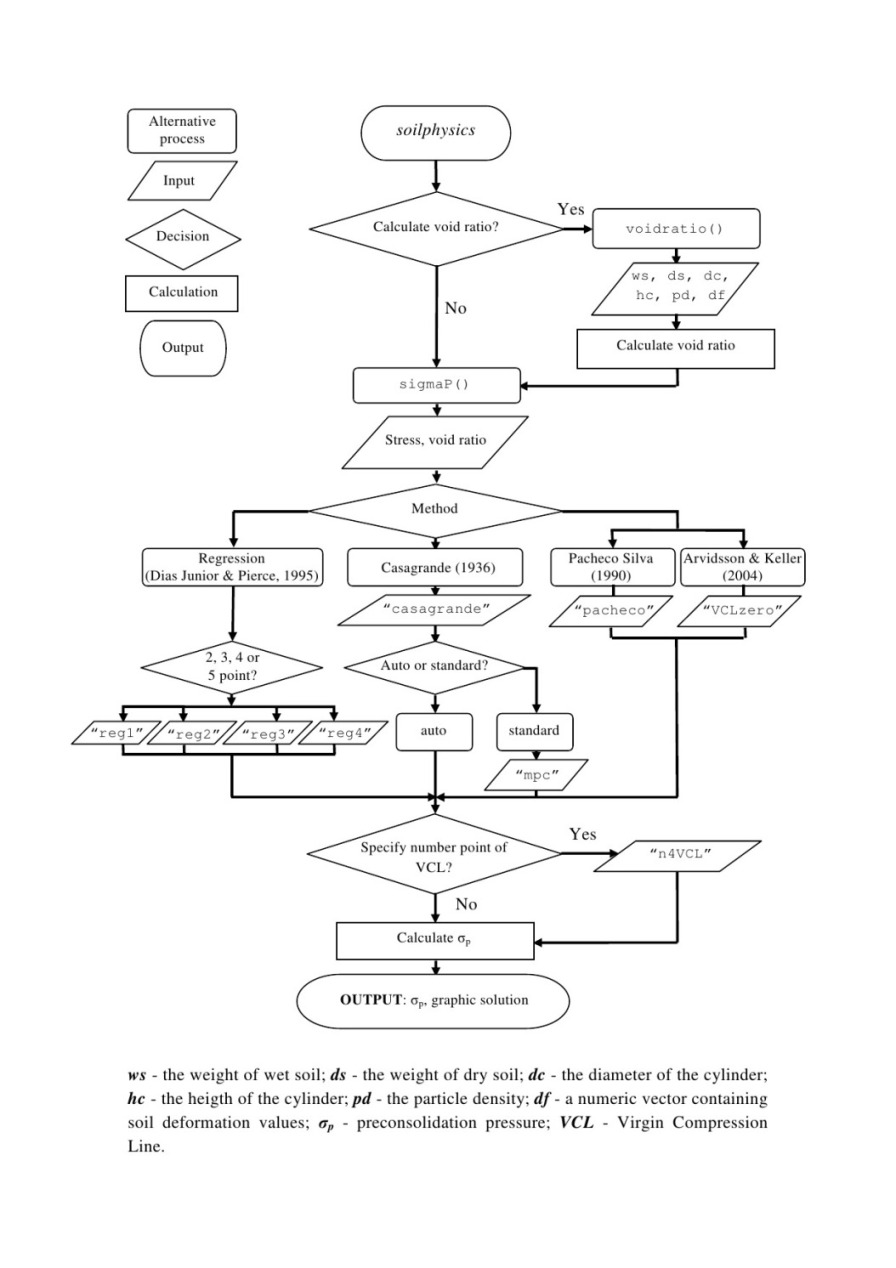
Value
A list of
sigmaP |
the preconsolidation stress. |
method |
the method used as argument. |
mcp |
the maximum curvature point in log10 scale of |
CI |
the compression index. |
SI |
the swelling index. |
Author(s)
Anderson Rodrigo da Silva <anderson.agro@hotmail.com>
References
ABNT - Associacao Brasileira de Normas Tecnicas. (1990). Ensaio de adensamento unidimensional: NBR 12007. Rio de Janeiro. 13p.
Arvidsson, J.; Keller, T. (2004). Soil precompression stress I. A survey of Swedish arable soils. Soil & Tillage Research, 77:85-95.
Bowles, J. A. (1986). Engineering Properties of Soils and their Measurements, 3rd edition. McGraw-Hill Book Company, Inc. NY, 218pp.
Casagrande, A. (1936). The determination of the pre-consolidation load and its practical significance. In: Proceedings of the International Conference on Soil Mech. and Found. Eng. (ICSMFE), Cambridge, MA, 22-26 June 1936, vol. 3. Harvard University, Cambridge, MA, USA, pp. 60-64.
Dias Junior, M. S.; Pierce, F. J. (1995). A simple procedure for estimating preconsolidation pressure from soil compression curves. Soil Technology, 8:139-151.
See Also
Examples
pres <- c(1, 12.5, 25, 50, 100, 200, 400, 800, 1600)
VR <- c(0.846, 0.829, 0.820, 0.802, 0.767, 0.717, 0.660, 0.595, 0.532)

plot(VR ~ log10(pres), type = "b") # find the 'mcp'
sigmaP(VR, pres, method = "casagrande", mcp = 1.6, n4VCL = 2)

# fitting the VCL
sigmaP(VR, pres, method = "casagrande", mcp = 1.6, n4VCL = 3)

# self-calculation of "mcp" argument for Casagrande method
sigmaP(VR, pres, method = "casagrande", n4VCL = 3)

# Pacheco method
sigmaP(VR, pres, method = "pacheco")

# Regression method
sigmaP(VR, pres, method = "reg3")

# End (not run)
Simulating Preconsolidation Stress
Description
Simulating preconsolidation pressure, compression and swelling indices, based on a multivariate Gaussian distribution for the parameters of the compression curve.
Usage
simSigmaP(voidratio, stress,
	what.out = c("sigmaP", "CI", "SI"),
	method = c("casagrande", "VCLzero", "reg1", "reg2", "reg3", "reg4", "pacheco"),
	n4VCL = 3, nsim = 100)
Arguments
voidratio |
a numeric vector containing void ratio (or bulk density) values. |
stress |
a numeric vector containing the applied stress sequence. |
what.out |
a character indicating which |
method |
a character vector indicating which methods should be used. |
n4VCL |
the number of points for calculating the slope of the soil Virgin Compression Line (VCL), which is obtained by linear regression. Default is 3. |
nsim |
the number of simulations. Default is 100. Warning: it may cause time demanding. |
Value
A numeric matrix containing the simulated values for each method selected as input.
Author(s)
Anderson Rodrigo da Silva <anderson.agro@hotmail.com>
See Also
Examples
# input data: stress and void ratio
pres <- c(1, 12.5, 25, 50, 100, 200, 400, 800, 1600)
VR <- c(1.43, 1.41, 1.40, 1.39, 1.35, 1.31, 1.25, 1.18, 1.12)

# simulation (may take a few seconds)
simres <- simSigmaP(VR, pres, nsim = 30)
head(simres)

# plot percentile confidence intervals
ci <- plotCIsigmaP(simres, conf.level = 0.95,
	shade.col = "blue", ordered = TRUE)
print(ci)

# End (Not run)
LLWR Data Set
Description
Data set presented by Leao et al. (2005), for determining the Least Limiting Water Range.
Usage
data(skp1994)Format
A data frame with 64 observations on the following 4 variables:
BDa numeric vector containing soil bulk density values, in Mg/m3.
Wa numeric vector containing volumetric water content values, in m3/m3.
PRa numeric vector containing penetration resistance values, in MPa.
ha numeric vector containing matric head values, in cm.
Source
Leao et al. (2005). An Algorithm for Calculating the Least Limiting Water Range of Soils. Agronomy Journal, 97:1210-1215.
Examples
data(skp1994)
summary(skp1994)
Soil deformation by O'Sullivan and Robertson (1996)
Description
It calculates bulk density variation as a function of the applied mean normal stress using critical state theory, by O'Sullivan and Robertson (1996).
Usage
soilDeformation(stress, p.density, iBD, N, CI, k, k2, m, graph = FALSE, ...)
Arguments
stress |
a numeric vector containing the values of mean normal stress, kPa; Note that stress can also be a vector of length 1. |
p.density |
a numeric vector containing the values of particle density to each stress, |
iBD |
a numeric vector containing the values of initial bulk density to each stress, |
N |
the specific volume at p = 1 kPa, to each stress |
CI |
the compression index, to each stress; check details |
k |
the recompression index, to each stress; check details |
k2 |
the slope of the steeper recompression line to each stress (similar to the k' in O'Sullivan and Robertson (1996) model); check details |
m |
the value that separates yield line and VCL to each stress; check details |
graph |
logical; shall soilDeformation plot the graph model (only the first parameters set is ploted)? |
... |
further graphical arguments. See par. |
Details
The specific volume (v) is given as v=PD/BD, where PD is particle density and BD is the bulk
density. Please, check each parameter from O'Sullivan and Robertson (1996) model in the figure below.
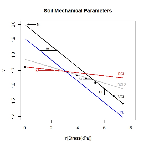
Value
A list of
iBD |
initial bulk density, |
fBD |
final bulk density, |
vi |
initial specific volume |
vf |
final specific volume |
I |
variation of soil bulk density ( |
Author(s)
Renato Paiva de Lima <renato_agro_@hotmail.com>
Anderson Rodrigo da Silva <anderson.agro@hotmail.com>
Alvaro Pires da Silva <apisilva@usp.br>
References
O'Sullivan, M.F.; Robertson, E.A.G. 1996. Critical state parameters from intact samples of two agricultural soils. Soil and Tillage Research, 39:161-173.
Keller, T.; Defossez, P.; Weisskopf, P.; Arvidsson, J.; Richard, G. 2007. SoilFlex: a model for prediction of soil stresses and soil compaction due to agricultural field traffic including a synthesis of analytical approaches. Soil and Tillage Research, 93:391-411.
Examples
# EXAMPLE 1
soilDeformation(stress = 300,
                p.density = 2.67,
	        iBD = 1.55,
                N = 1.9392,
                CI = 0.06037,
                k = 0.00608,
                k2 = 0.01916,
                m = 1.3,graph=TRUE,ylim=c(1.4,1.8))

# EXEMPLE 2 (combining it with soil stress)
stress <- stressTraffic(inflation.pressure=200,
	        recommended.pressure=200,
	        tyre.diameter=1.8,
	        tyre.width=0.4,
	        wheel.load=4000,
	        conc.factor=c(4,5,5,5,5,5),
                layers=c(0.05,0.1,0.3,0.5,0.7,1),
	        plot.contact.area = FALSE)

stress.mean <- stress$Stress$sigma_mean
layers <- stress$Stress$Layers
n <- length(layers)

def <- soilDeformation(stress = stress.mean,
                p.density = rep(2.67, n),
	        iBD = rep(1.55,n),
                N = rep(1.9392,n),
                CI = rep(0.06037,n),
                k = rep(0.00608,n),
                k2 = rep(0.01916,n),
                m = rep(1.3,n),graph=TRUE,ylim=c(1.4,1.8))

# Graph
plot(x = 1, y = 1,
     xlim=c(1.4,1.7),ylim=c(1,0),xaxt = "n",
     ylab = "Soil Depth",xlab ="", type="l", main="")
axis(3)
mtext("Bulk Density",side=3,line=2.5)

initial.BD <- def$iBD
final.BD <- def$fBD
points(x=initial.BD, y=layers, type="l")
points(x=initial.BD, y=layers,pch=15)
points(x=final.BD, y=layers, type="l", col=2)
points(x=final.BD, y=layers,pch=15, col=2)

# End (not run)
Estimation of precompression stress by Severiano et al. (2013)
Description
It calculates the precompression stress using the pedo-transfer function from Severiano et al. (2013)
Usage
soilStrength(clay.content, matric.suction = NULL, water.content = NULL)
Arguments
clay.content |
a numeric vector containing the values of clay for each soil layer, %. Note that it can also be a unique value. |
matric.suction |
a numeric vector containing the values of matric suction for each clay content, kPa. |
water.content |
a numeric vector containing the values of water content for each clay content, |
Details
Intervals of soil water content/matric suction to be used as input for estimating soil strength according to Severiano et al. (2013).
Value
A two-columns data frame:
Pc |
the precompression stress (Severiano et al. 2013) |
LL.Pc |
the lower limit of precompression stress in acoording to the Terranimo model criteria (see Stettler et al. 2014). Note: LL.Pc = Pc*0.5 |
UL.Pc |
the upper limit of precompression stress in acoording to the Terranimo model criteria (see Stettler et al. 2014). Note: UL.Pc = Pc*1.1 |
Author(s)
Renato Paiva de Lima <renato_agro_@hotmail.com>
Anderson Rodrigo da Silva <anderson.agro@hotmail.com>
Alvaro Pires da Silva <apisilva@usp.br>
References
Severiano, E.C; Oliveira, G.C.; Dias Junior, M.S.; Curi, N.C.; Costa, K. A.P.; Carducci, C.E. 2013. Preconsolidation pressure, soil water retention characteristics, and texture of Latosols in the Brazilian Cerrado. Soil Research, 51:193-202.
Stettler, M., Keller, T., Weisskopf, P., Lamande, M., Lassen, P., Schjonning, P., 2014. Terranimo - a web-based tool for evaluating soil compaction. Landtechnik, 69:132-137.
See Also
Examples
# EXEMPLE 1 (using water content)
soilStrength(clay.content=c(25,28,30,30,30),
             water.content = c(0.26,0.27,0.29,0.32,0.32))


# EXEMPLE 2 (using matric suction)
soilStrength(clay.content=c(25,28,30,30,30),
             matric.suction = c(100,330,1000,3000,5000))


# EXAMPLE 3 (combining it with soil stress)
stress <- stressTraffic(inflation.pressure=200,
	        recommended.pressure=200,
	        tyre.diameter=1.8,
	        tyre.width=0.4,
	        wheel.load=4000,
	        conc.factor=c(4,5,5,5,5,5),
                layers=c(0.05,0.1,0.3,0.5,0.7,1),
	        plot.contact.area = FALSE)

strength <- soilStrength(clay.content=c(25,28,30,30,30,30),
              matric.suction = c(30,100,100,100,200,200))


# Graph
plot(x = 1, y = 1,
     xlim=c(0,300),ylim=c(1,0),xaxt = "n",
     ylab = "Soil Depth",xlab ="", type="l", main="")
axis(3)
mtext("Vertical Stress",side=3,line=2.5)

stressz <- stress$Stress$sigma_vertical
layers <- stress$Stress$Layers
points(x=stressz, y=layers, type="l")

# Green zone
x0 <- strength$LL.Pc
x1 <- rep(0,length(layers))
y0 <- layers
y1 <- rev(layers)
polygon(x=c(x0,x1), y = c(y0,y1),density = NA,
       col=rgb(red=0, green=1, blue=0, alpha=0.3))

# Yellow zone
x0 <- strength$UL.Pc
x1 <- rev(strength$LL.Pc)
y0 <- layers
y1 <- rev(layers)
polygon(x=c(x0,x1), y = c(y0,y1),density = NA,
       col=rgb(red=1, green=1, blue=0, alpha=0.3))

# Red zone
x0 <- rep(300,length(layers))
x1 <- rev(strength$UL.Pc)
y0 <- layers
y1 <- rev(layers)
polygon(x=c(x0,x1), y = c(y0,y1),density = NA,
       col=rgb(red=1, green=0, blue=0, alpha=0.3))

# End (not run)
Estimation of precompression stress by Schjonning and Lamande (2018)
Description
It calculates the precompression stress using the pedo-transfer function from Schjonning and Lamande (2018)
Usage
soilStrength2(bulk.density, matric.suction, clay.content)
Arguments
clay.content |
a numeric vector containing the values of clay content, |
matric.suction |
a numeric vector containing the values of matric suction, hPa |
bulk.density |
a numeric vector containing the values of soil bulk density, |
Details
The function returns 0 for soil properties values beyond the range for which the function was built.
Value
PC |
the precompression stress |
Author(s)
Renato Paiva de Lima <renato_agro_@hotmail.com> Anderson Rodrigo da Silva <anderson.agro@hotmail.com>
References
Schjonning, P.; Lamande, M., 2018. Models for prediction of soil precompression stress from readily available soil properties. Geoderma, 320:115-125.
See Also
Examples
# EXAMPLE 1

soilStrength2(bulk.density=1.46, matric.suction=100, clay.content=0.3)


# EXAMPLE 2

matric.suction <- seq(from=60,to=1000,len=50) # range of matric suction from 60 to 1200 hPa
out <- soilStrength2(bulk.density=1.46, matric.suction=matric.suction, clay.content=0.3)
plot(x=matric.suction,y=out,
     ylab="Precompression stress (kPa)", xlab="Matric suction (hPa)")

# End (not run)
Estimation of precompression stress by Saffih-Hdadi et al. (2009)
Description
It calculates the precompression stress using the pedo-transfer function from Saffih-Hdadi et al. (2009)
Usage
soilStrength3(bulk.density, water.content,
              texture=c("VeryFine","Fine","MediumFine","Medium","Coarse"))
Arguments
bulk.density |
a numeric vector containing the values of soil bulk density, |
water.content |
a numeric vector containing the values of gravimetric water content, |
texture |
the soil texture group. See exemples |
Details
The function returns 0 for soil properties values beyond the range for which the function was built.
Value
PC |
the precompression stress |
Author(s)
Renato Paiva de Lima <renato_agro_@hotmail.com> Anderson Rodrigo da Silva <anderson.agro@hotmail.com>
References
Saffih-Hdadi, K.; Defossez, P.; Richard, G.; Cui, Y. J.; Tang, A. M.; Chaplain, V, 2009. A method for predicting soil susceptibility to the compaction of surface layers as a function of water content and bulk density Geoderma, 115: 96-103.
See Also
Examples
# EXAMPLE 1

soilStrength3(bulk.density=1.1, water.content=40, texture="VeryFine")
soilStrength3(bulk.density=1.2, water.content=20, texture="Fine")
soilStrength3(bulk.density=1.3, water.content=15, texture="MediumFine")
soilStrength3(bulk.density=1.4, water.content=15, texture="Medium")
soilStrength3(bulk.density=1.5, water.content=10, texture="Coarse")

# End (not run)
Estimation of precompression stress by Lebert and Horn (1991)
Description
It calculates the soil strength through precompression stress using the pedo-transfer function from Lebert and Horn (1991)
Usage
soilStrength4(BD=1.55,AC=10,AWC=15,PWP=26,Ks=0.29,
              OM=1.5,C=30,phi=36,texture="Clay>35", pF=1.8)
Arguments
BD |
a numeric vector containing the values of soil bulk density, |
AC |
a numeric vector containing the values of volumetric air capacity at the specified pF, |
AWC |
a numeric vector containing the values of volumetric available water at the specified pF, |
PWP |
a numeric vector containing the values of volumetric non available water capacity (pF > 4.2), |
Ks |
a numeric vector containing the values of saturated hydraulic conductivity, |
OM |
a numeric vector containing the values of organic matter, |
C |
a numeric vector containing the values of cohesion at the specified pF, kPa |
phi |
a numeric vector containing the values of angle of internal friction at the specified pF, degree |
texture |
the soil texture classification. See details |
pF |
the '1.8' or '2.5' value pF |
Details
The function returns '0' for soil properties values beyond the range for which the function was built. The default for this function is the values given in the application example by Horn and Fleige (2003). In the 'texture' argument, the user must pass the textural classification 'Sand','SandLoam', 'Silt', 'Clay<35' or 'Clay>35'. See examples.
Value
PC |
the precompression stress |
Author(s)
Renato Paiva de Lima <renato_agro_@hotmail.com> Anderson Rodrigo da Silva <anderson.agro@hotmail.com>
References
Lebert, M., Horn, R. (1991) A method to predict the mechanical strength of agricultural soils. Soil and Tillage Research, 19: 275-256.
Horn, R., Fleige, H. (2003) A method for assessing the impact of load on mechanical stability and on physical properties of soils. Soil and Tillage Research, 73: 89-99.
See Also
Examples
soilStrength4(BD=1.55,AC=10,AWC=15,PWP=26,Ks=0.29,OM=1.5,
              C=30,phi=36,texture="Clay>35", pF=1.8) # Exemple from Horn and Fleige (2003), Table 7

# End (not run)
Estimation of precompression stress by Imhoff et al. (2004)
Description
It calculates the soil strength using precompression stress using the pedo-transfer function from Imhoff et al. (2004)
Usage
soilStrength5(bulk.density, water.content, clay.content)
Arguments
bulk.density |
a numeric vector containing the values of soil bulk density, |
water.content |
a numeric vector containing the values of water content, (g/g) |
clay.content |
a numeric vector containing the values of clay content, |
Details
The function returns 0 for soil properties values beyond the range for which the function was built.
Value
PC |
the precompression stress |
Author(s)
Renato Paiva de Lima <renato_agro_@hotmail.com> Anderson Rodrigo da Silva <anderson.agro@hotmail.com>
References
Imhoff, S., Da Silva, A. P., Fallow, D. (2004) Susceptibility to Compaction, Load Support Capacity, and Soil Compressibility of Hapludox. Soil Science Society of America Journal, 68: 17-24.
See Also
Examples
# EXAMPLE 1

soilStrength5(clay.content=60, water.content=0.30, bulk.density=1.25)
soilStrength5(clay.content=35, water.content=0.23, bulk.density=1.40)
soilStrength5(clay.content=20, water.content=0.10, bulk.density=1.60)


# EXAMPLE 2
water.content <- seq(0.1,0.30,len=20) # range of water content from 0.1 to 0.30 (g g^-1)
out <- soilStrength5(clay.content=20, water.content=water.content , bulk.density=1.60)
plot(x=water.content,y=out,
     ylab="Precompression stress (kPa)", xlab="Water content")


# End (not run)
Soil Water Retention, based on the van Genuchten's (1980) formula
Description
Function to calculate the soil water content based on the van Genuchten's (1980) formula:
\theta = \theta_R + (\theta_S - \theta_R)(1 + (\alpha x)^n)^{-m}
Usage
soilwater(x, theta_R, theta_S, alpha, n, m = 1 - 1/n,
    saturation.index = FALSE)
Arguments
x |
the matric potential. |
theta_R |
the residual water content. |
theta_S |
the water content at saturation. |
alpha |
a scale parameter of the van Genuchten's formula. |
n |
a shape parameter in van Genuchten's formula. |
m |
a shape parameter in van Genuchten's Formula. Default is |
saturation.index |
logical; if FALSE (default) the outcome is the soil water content, otherwise the saturation index is returned. |
Value
The the soil water content or the saturation index (a value between 0 and 1).
Author(s)
Anderson Rodrigo da Silva <anderson.agro@hotmail.com> (code adapted from the function swc(), package soilwater (Cordano et al., 2012).)
References
Genuchten, M. T. van. (1980). A closed form equation for predicting the hydraulic conductivity of unsaturated soils. Soil Science Society of America Journal, 44:892-898.
Mualem, Y. (1976). A new model for predicting the hydraulic conductivity of unsaturated porous media. Water Resources Research, 12:513-522.
See Also
Examples
# example 1
soilwater(x = 0.1, theta_R = 0.06, theta_S = 0.25, alpha = 21, n = 2.08)
curve(soilwater(x, theta_R = 0.06, theta_S = 0.25, alpha = 21, n = 2.08))

# example 2 (punctual predictions)
p <- seq(0, 1, length.out = 10)
m <- soilwater(x = p, theta_R = 0.06, theta_S = 0.25,
	alpha = 21, n = 2.08)
points(m ~ p, type = "b", col = "red")

# End (not run)
Soil Water Retention, based on the Groenevelt & Grant (2004) formula
Description
Function to calculate the soil water content based on the Groenevelt & Grant (2004) model. It is based on thermodynamic principles. Therefore, it is appropriate for the case in which thermodynamic equilibrium has been attained by diffusion of water. In this case, the water retention curve is given by:
\theta = k_1 \exp(-k_0 / x_0^n) - k_1 \exp(-k_0 / x^n)
where x = log h (pore water suction), and h is in units of hPa
Usage
soilwater2(x, x0 = 6.653, k0, k1, n)
Arguments
x |
a numeric vector containing pF values. |
x0 |
the value of pF (pore water suction) at which the soil water content becomes zero. The default is 6.653. |
k0 |
a parameter value. |
k1 |
a parameter value. |
n |
a parameter value. |
Value
The the soil water content.
Author(s)
Anderson Rodrigo da Silva <anderson.agro@hotmail.com>
References
Groenevelt & Grant (2004). A newmodel for the soil-water retention curve that solves the problem of residualwater contents. European Journal of Soil Science, 55:479-485.
See Also
Examples
pF <- 0:7
soilwater2(pF, k0 = 1.867, k1 = 0.426, n = 2.358)

# End (not run)
Soil Water Retention, based on the Dexter's (2008) formula
Description
Function to calculate the soil water content based on the Dexter's (2008) formula. It is based on the segregation of pore space in two categories what are called bi-modal pore size distributions. In this model, the pore space is divided into two parts: the textural porosity which occurs between the primary mineral particles, and the structural porosity which occurs between micro aggregates and/or any other compound particles. This is called the double-exponential (DE) water retention equation, given by:
\theta = \theta_R + a_1 \exp(-x/p_1) + a_2 \exp(-x/p_2)
where \theta is the gravimetric water content.
Usage
soilwater3(x, theta_R, a1, p1, a2, p2)
Arguments
x |
a numeric vector containing the values of applied air pressure. |
theta_R |
a parameter that represents the residual water content. |
a1 |
a parameter that represents the drainable part of the textural pore space in units of gravimetric water content at saturation. |
p1 |
a parameter that represents the applied air pressures characteristic for displacement of water from the textural pore space. |
a2 |
a parameter that represents the total structural pore space in units of gravimetric water content at saturation. |
p2 |
a parameter that represents the applied air pressure that is characteristic for displacing water from the structural pores. |
Value
The the soil water content.
Author(s)
Anderson Rodrigo da Silva <anderson.agro@hotmail.com>
References
Dexter et al. (2008). A user-friendly water retention function that takes account of the textural and structural pore spaces in soil. Geoderma, 143:243-253.
See Also
fitsoilwater3, soilwater, soilwater2
Examples
soilwater3(x = 0, theta_R = 0.058, a1 = 0.233, p1 = 3.274, a2 = 0.070, p2 = 1.78)
soilwater3(x = 3, theta_R = 0.058, a1 = 0.233, p1 = 3.274, a2 = 0.070, p2 = 1.78)
soilwater3(x = 4, theta_R = 0.058, a1 = 0.233, p1 = 3.274, a2 = 0.070, p2 = 1.78)

# End (not run)
Soil Water Retention, based on Power Models
Description
Function to calculate the soil water content based on the following formulas:
\theta = \exp(a + b*Bd) \psi^c
(Silva et al., 1994)
\theta = a \psi^c
(Ross et al., 1991)
where \theta is the soil water content.
Usage
soilwater4(psi, Bd, a, b, c, model = c("Silva", "Ross"))
Arguments
psi |
a numeric vector containing values of water potential (Psi). |
Bd |
a numeric vector containing values of dry bulk density. |
a |
a model-fitting parameter. See details. |
b |
a model-fitting parameter. See details. |
c |
a model-fitting parameter. See details. |
model |
a character; the model to be used for calculating the soil water content. It must be one of the
two: |
Details
The parameters "a" and "c" have the same meaning in both models, but be aware that the parameter "a" of the model employed by Silva et al. (1994) is parameter "a" of the Ross et al. (1991) in a log10 scale.
Value
The the soil water content.
Author(s)
Anderson Rodrigo da Silva <anderson.agro@hotmail.com>
References
Ross et al. (1991). Equation for extending water-retention curves to dryness. Soil Science Society of America Journal, 55:923-927.
Silva et al. (1994). Characterization of the least limiting water range of soils. Soil Science Society of America Journal, 58:1775-1781.
See Also
fitsoilwater4, soilwater, soilwater2, soilwater3
Examples
# End (not run)
Soil Water Retention, based on the modified van Genuchten's formula
Description
Function to calculate the soil water content based on the modified van Genuchten's formula, as suggested by Pierson and Mulla (1989):
\theta = \theta_R + (\theta_S - \theta_R)(1 + (\alpha x)^n)^{-m} + b_0 + b_1 x + b_2 * x^2
Usage
soilwater5(x, theta_R, theta_S, alpha, n, m = 1 - 1/n, b0, b1, b2)
Arguments
x |
the matric potential. |
theta_R |
the residual water content. |
theta_S |
the water content at saturation. |
alpha |
a scale parameter of the van Genuchten's formula. |
n |
a shape parameter in van Genuchten's formula. |
m |
a shape parameter in van Genuchten's Formula. Default is |
b0 |
a parameter added to the van Ganuchten's formula. |
b1 |
a parameter added to the van Ganuchten's formula. |
b2 |
a parameter (of quadratic term) added to the van Ganuchten's formula. |
Value
The the soil water content or the saturation index (a value between 0 and 1).
Author(s)
Anderson Rodrigo da Silva <anderson.agro@hotmail.com>
References
Pierson, F.B.; Mulla, D.J. (1989) An Improved Method for Measuring Aggregate Stability of a Weakly Aggregated Loessial Soil. Soil Sci. Soc. Am. J., 53:1825–1831.
See Also
Examples
soilwater5(x = 20, theta_R = 0.2735, theta_S = 0.478, alpha = 0.1029,
	n = 9.45, b0 = 0.2278, b1 = -0.0165, b2 = 0.000248)
curve(soilwater5(x, theta_R = 0.2735, theta_S = 0.478, alpha = 0.1029,
	n = 9.45, b0 = 0.2278, b1 = -0.0165, b2 = 0.000248),
	from = 0, to = 40,
	ylab = "Water content",
	xlab = "Matric potential")

# End (Not run)
Predicting Soil Stress Due to Agricultural Trafficability
Description
Contact area, stress distribuition and stress propagation based on the SoilFlex model (Keller 2005; Keller et al. 2007) are calculated.
Usage
stressTraffic(inflation.pressure, recommended.pressure, tyre.diameter,
    tyre.width, wheel.load, conc.factor, layers, plot.contact.area = FALSE, ...)
Arguments
inflation.pressure |
tyre inflation pressure, kPa |
recommended.pressure |
recommended tyre inflation pressure at given load, kPa |
tyre.diameter |
overall diameter of the unloaded tyre, m |
tyre.width |
tyre width, m |
wheel.load |
wheel load, kg |
conc.factor |
concentration factor; a numeric vector ranging from 3 (wet soil) to 6 (dry soil), depending on water content. |
layers |
a numeric vector containing values of depth (in meters) for the soil layers. Note that layers can also be a unique value |
plot.contact.area |
logical; shall |
... |
further graphical arguments. See par. |
Value
A list of
Area |
Contact area parameters. |
Loads |
Estimated wheel loads. |
Stress |
Stress propagation into soil; sigma_vertical: vertical stress; sigma_mean: mean normal stress |
stress.matrix |
The matrix of applied stress at a specific depth and radial distance from the tyre centre. |
fZStress |
The function of stress propagation in z direction (vertical stress). |
fmeanStress |
The function of mean normal stress propagation. |
fStress |
The function of stress propagation. |
fXStress |
The function of stress propagation in x (footprint length or driving) direction. |
fYStress |
The function of stress propagation in y (tire width) direction. |
Author(s)
Renato Paiva de Lima <renato_agro_@hotmail.com>
Anderson Rodrigo da Silva <anderson.agro@hotmail.com>
Alvaro Pires da Silva <apisilva@usp.br>
References
Keller, T. 2005. A model to predict the contact area and the distribution of vertical stress below agricultural tyres from readily-available tyre parameters. Biosyst. Eng. 92, 85-96.
Keller, T.; Defossez, P.; Weisskopf, P.; Arvidsson, J.; Richard, G. 2007. SoilFlex: a model for prediction of soil stresses and soil compaction due to agricultural field traffic including a synthesis of analytical approaches. Soil and Tillage Research 93, 391-411.
Examples
stress <- stressTraffic(inflation.pressure=200,
	   recommended.pressure=200,
	   tyre.diameter=1.8,
	   tyre.width=0.4,
	   wheel.load=4000,
	   conc.factor=c(4,5,5,5,5,5),
           layers=c(0.05,0.1,0.3,0.5,0.7,1),
	   plot.contact.area = TRUE)

stress

# Building a fancier plot for the contact area
# library(fields)
# image.plot(x = as.numeric(rownames(stress$stress.matrix)),
#	       y = as.numeric(colnames(stress$stress.matrix)),
#	       z = stress$stress.matrix,
#	       xlab="Tyre footprint length (m)", ylab="Tyre width (m)")
# End (not run)

# Stress Propagation
# Vertical Stress
stress.v <- stress$Stress$sigma_vertical
layers <- stress$Stress$Layers
plot(x = 1, y = 1, xlim=c(0,300),ylim=c(1,0),xaxt = "n",
     ylab = "Soil Depth",xlab ="", type="l", main="")
axis(3)
mtext("Stress (kPa)",side=3,line=2.5)
lines(x=stress.v, y=layers)

# Mean normal stress
stress.p <- stress$Stress$sigma_mean
lines(x=stress.p, y=layers, lty=2)
legend("bottomright", c("Vertical stress", "Normal mean stress"), lty = 1:2)

# End (not run)
Void Ratio
Description
A function to calculate the soil void ratio.
Usage
voidratio(wetsoil, drysoil, diam.cylinder, height.cylinder,
    dens.particle, deformation)
Arguments
wetsoil |
the weight of wet soil. |
drysoil |
the weight of dry soil. |
diam.cylinder |
the diameter of the cylinder. |
height.cylinder |
the heigth of the cylinder. |
dens.particle |
the particle density. |
deformation |
a numeric vector containing soil deformation values. |
Value
A numeric vector with same length of deformation containig void ratio values.
Author(s)
Anderson Rodrigo da Silva <anderson.agro@hotmail.com>
See Also
Examples
def <- c(0, 0.0230, 0.0352, 0.0605, 0.1070, 0.1750, 0.2525, 0.3395, 0.4250)
pres <- c(1, 12.5, 25, 50, 100, 200, 400, 800, 1600)
VR <- voidratio(wetsoil = 170.62, drysoil = 134.08, diam.cylinder = 6.95,
               height.cylinder = 2.5, dens.particle = 2.61, def)
VR

plot(VR ~ pres, type = "b",
	ylab = "Void ratio",
	xlab = "Applied stress (kPa)",
	main = "Compression curve",
	log = "x")

# End (not run)