Title:	Utilities for Scoring and Assessing Predictions
Version:	2.1.1
Language:	en-GB
Description:	Facilitate the evaluation of forecasts in a convenient framework based on data.table. It allows user to to check their forecasts and diagnose issues, to visualise forecasts and missing data, to transform data before scoring, to handle missing forecasts, to aggregate scores, and to visualise the results of the evaluation. The package mostly focuses on the evaluation of probabilistic forecasts and allows evaluating several different forecast types and input formats. Find more information about the package in the Vignettes as well as in the accompanying paper, <doi:10.48550/arXiv.2205.07090>.
License:	MIT + file LICENSE
Encoding:	UTF-8
LazyData:	true
Imports:	checkmate, cli, data.table (≥ 1.16.0), ggplot2 (≥ 3.4.0), methods, Metrics, purrr, scoringRules (≥ 1.1.3), stats
Suggests:	ggdist, kableExtra, knitr, magrittr, rmarkdown, testthat (≥ 3.1.9), vdiffr
Config/Needs/website:	r-lib/pkgdown, amirmasoudabdol/preferably
Config/testthat/edition:	3
RoxygenNote:	7.3.2
URL:	https://doi.org/10.48550/arXiv.2205.07090, https://epiforecasts.io/scoringutils/, https://github.com/epiforecasts/scoringutils
BugReports:	https://github.com/epiforecasts/scoringutils/issues
VignetteBuilder:	knitr
Depends:	R (≥ 4.1)
NeedsCompilation:	no
Packaged:	2025-06-25 22:05:16 UTC; nikos
Author:	Nikos Bosse [aut, cre], Sam Abbott [aut], Hugo Gruson [aut], Johannes Bracher [ctb], Toshiaki Asakura [ctb], James Mba Azam [ctb], Sebastian Funk [aut], Michael Chirico [ctb]
Maintainer:	Nikos Bosse <nikosbosse@gmail.com>
Repository:	CRAN
Date/Publication:	2025-06-25 22:20:02 UTC

scoringutils: Utilities for Scoring and Assessing Predictions

Description

Facilitate the evaluation of forecasts in a convenient framework based on data.table. It allows user to to check their forecasts and diagnose issues, to visualise forecasts and missing data, to transform data before scoring, to handle missing forecasts, to aggregate scores, and to visualise the results of the evaluation. The package mostly focuses on the evaluation of probabilistic forecasts and allows evaluating several different forecast types and input formats. Find more information about the package in the Vignettes as well as in the accompanying paper, doi:10.48550/arXiv.2205.07090.

Author(s)

Maintainer: Nikos Bosse nikosbosse@gmail.com (ORCID)

Authors:

• Sam Abbott contact@samabbott.co.uk (ORCID)

• Hugo Gruson hugo.gruson+R@normalesup.org (ORCID)

• Sebastian Funk sebastian.funk@lshtm.ac.uk

Other contributors:

• Johannes Bracher johannes.bracher@kit.edu (ORCID) [contributor]

• Toshiaki Asakura toshiaki.asa9ra@gmail.com (ORCID) [contributor]

• James Mba Azam james.azam@lshtm.ac.uk (ORCID) [contributor]

• Michael Chirico michaelchirico4@gmail.com (ORCID) [contributor]

See Also

Useful links:

• doi:10.48550/arXiv.2205.07090

• https://epiforecasts.io/scoringutils/

• https://github.com/epiforecasts/scoringutils

• Report bugs at https://github.com/epiforecasts/scoringutils/issues

Add relative skill scores based on pairwise comparisons

Description

Adds a columns with relative skills computed by running pairwise comparisons on the scores. For more information on the computation of relative skill, see get_pairwise_comparisons(). Relative skill will be calculated for the aggregation level specified in by.

Usage

add_relative_skill(
  scores,
  compare = "model",
  by = NULL,
  metric = intersect(c("wis", "crps", "brier_score"), names(scores)),
  baseline = NULL,
  ...
)

Arguments

Absolute error of the median (quantile-based version)

Description

Compute the absolute error of the median calculated as

|\text{observed} - \text{median prediction}|

The median prediction is the predicted value for which quantile_level == 0.5. The function requires 0.5 to be among the quantile levels in quantile_level.

Usage

ae_median_quantile(observed, predicted, quantile_level)

Arguments

Value

Numeric vector of length N with the absolute error of the median.

Input format

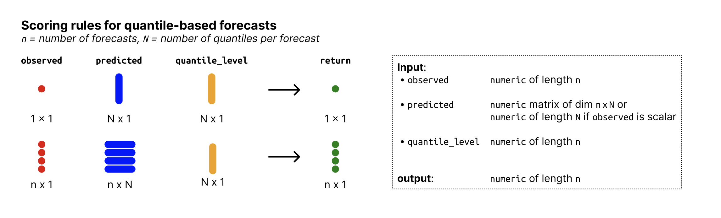
Overview of required input format for quantile-based forecasts

See Also

ae_median_sample()

Examples

observed <- rnorm(30, mean = 1:30)
predicted_values <- replicate(3, rnorm(30, mean = 1:30))
ae_median_quantile(
  observed, predicted_values, quantile_level = c(0.2, 0.5, 0.8)
)

Absolute error of the median (sample-based version)

Description

Absolute error of the median calculated as

|\text{observed} - \text{median prediction}|

where the median prediction is calculated as the median of the predictive samples.

Usage

ae_median_sample(observed, predicted)

Arguments

Value

Numeric vector of length n with the absolute errors of the median.

Input format

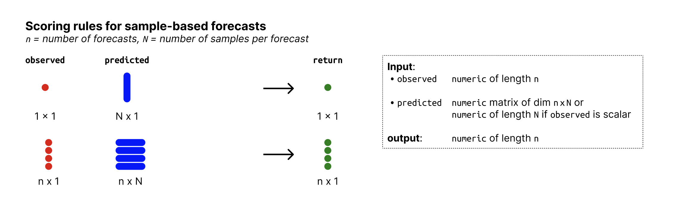
Overview of required input format for sample-based forecasts

See Also

ae_median_quantile()

Examples

observed <- rnorm(30, mean = 1:30)
predicted_values <- matrix(rnorm(30, mean = 1:30))
ae_median_sample(observed, predicted_values)

Apply a list of functions to a data table of forecasts

Description

This helper function applies scoring rules (stored as a list of functions) to a data table of forecasts. apply_metrics is used within score() to apply all scoring rules to the data. Scoring rules are wrapped in run_safely() to catch errors and to make sure that only arguments are passed to the scoring rule that are actually accepted by it.

Usage

apply_metrics(forecast, metrics, ...)

Arguments

Value

A data table with the forecasts and the calculated metrics.

Create a forecast object for binary forecasts

Description

Process and validate a data.frame (or similar) or similar with forecasts and observations. If the input passes all input checks, those functions will be converted to a forecast object. A forecast object is a data.table with a class forecast and an additional class that depends on the forecast type.

The arguments observed, predicted, etc. make it possible to rename existing columns of the input data to match the required columns for a forecast object. Using the argument forecast_unit, you can specify the columns that uniquely identify a single forecast (and thereby removing other, unneeded columns. See section "Forecast Unit" below for details).

Usage

as_forecast_binary(data, ...)

## Default S3 method:
as_forecast_binary(
  data,
  forecast_unit = NULL,
  observed = NULL,
  predicted = NULL,
  ...
)

Arguments

Value

A forecast object of class forecast_binary

Required input

The input needs to be a data.frame or similar with the following columns:

• observed: factor with exactly two levels representing the observed values. The highest factor level is assumed to be the reference level. This means that corresponding value in predicted represent the probability that the observed value is equal to the highest factor level.

• predicted: numeric with predicted probabilities, representing the probability that the corresponding value in observed is equal to the highest available factor level.

For convenience, we recommend an additional column model holding the name of the forecaster or model that produced a prediction, but this is not strictly necessary.

See the example_binary data set for an example.

Forecast unit

In order to score forecasts, scoringutils needs to know which of the rows of the data belong together and jointly form a single forecasts. This is easy e.g. for point forecast, where there is one row per forecast. For quantile or sample-based forecasts, however, there are multiple rows that belong to a single forecast.

The forecast unit or unit of a single forecast is then described by the combination of columns that uniquely identify a single forecast. For example, we could have forecasts made by different models in various locations at different time points, each for several weeks into the future. The forecast unit could then be described as forecast_unit = c("model", "location", "forecast_date", "forecast_horizon"). scoringutils automatically tries to determine the unit of a single forecast. It uses all existing columns for this, which means that no columns must be present that are unrelated to the forecast unit. As a very simplistic example, if you had an additional row, "even", that is one if the row number is even and zero otherwise, then this would mess up scoring as scoringutils then thinks that this column was relevant in defining the forecast unit.

In order to avoid issues, we recommend setting the forecast unit explicitly, using the forecast_unit argument. This will simply drop unneeded columns, while making sure that all necessary, 'protected columns' like "predicted" or "observed" are retained.

See Also

Other functions to create forecast objects: as_forecast_nominal(), as_forecast_ordinal(), as_forecast_point(), as_forecast_quantile(), as_forecast_sample()

Examples

as_forecast_binary(
  example_binary,
  predicted = "predicted",
  forecast_unit = c("model", "target_type", "target_end_date",
                    "horizon", "location")
)

General information on creating a forecast object

Description

Process and validate a data.frame (or similar) or similar with forecasts and observations. If the input passes all input checks, those functions will be converted to a forecast object. A forecast object is a data.table with a class forecast and an additional class that depends on the forecast type.

The arguments observed, predicted, etc. make it possible to rename existing columns of the input data to match the required columns for a forecast object. Using the argument forecast_unit, you can specify the columns that uniquely identify a single forecast (and thereby removing other, unneeded columns. See section "Forecast Unit" below for details).

Arguments

Forecast unit

In order to score forecasts, scoringutils needs to know which of the rows of the data belong together and jointly form a single forecasts. This is easy e.g. for point forecast, where there is one row per forecast. For quantile or sample-based forecasts, however, there are multiple rows that belong to a single forecast.

The forecast unit or unit of a single forecast is then described by the combination of columns that uniquely identify a single forecast. For example, we could have forecasts made by different models in various locations at different time points, each for several weeks into the future. The forecast unit could then be described as forecast_unit = c("model", "location", "forecast_date", "forecast_horizon"). scoringutils automatically tries to determine the unit of a single forecast. It uses all existing columns for this, which means that no columns must be present that are unrelated to the forecast unit. As a very simplistic example, if you had an additional row, "even", that is one if the row number is even and zero otherwise, then this would mess up scoring as scoringutils then thinks that this column was relevant in defining the forecast unit.

In order to avoid issues, we recommend setting the forecast unit explicitly, using the forecast_unit argument. This will simply drop unneeded columns, while making sure that all necessary, 'protected columns' like "predicted" or "observed" are retained.

Common functionality for ⁠as_forecast_<type>⁠ functions

Description

Common functionality for ⁠as_forecast_<type>⁠ functions

Usage

as_forecast_generic(data, forecast_unit = NULL, ...)

Arguments

Details

This function splits out part of the functionality of ⁠as_forecast_<type>⁠ that is the same for all ⁠as_forecast_<type>⁠ functions. It renames the required columns, where appropriate, and sets the forecast unit.

Create a forecast object for nominal forecasts

Description

Process and validate a data.frame (or similar) or similar with forecasts and observations. If the input passes all input checks, those functions will be converted to a forecast object. A forecast object is a data.table with a class forecast and an additional class that depends on the forecast type.

The arguments observed, predicted, etc. make it possible to rename existing columns of the input data to match the required columns for a forecast object. Using the argument forecast_unit, you can specify the columns that uniquely identify a single forecast (and thereby removing other, unneeded columns. See section "Forecast Unit" below for details).

Usage

as_forecast_nominal(data, ...)

## Default S3 method:
as_forecast_nominal(
  data,
  forecast_unit = NULL,
  observed = NULL,
  predicted = NULL,
  predicted_label = NULL,
  ...
)

Arguments

Details

Nominal forecasts are a form of categorical forecasts and represent a generalisation of binary forecasts to multiple outcomes. The possible outcomes that the observed values can assume are not ordered.

Value

A forecast object of class forecast_nominal

Required input

The input needs to be a data.frame or similar for the default method with the following columns:

• observed: Column with observed values of type factor with N levels, where N is the number of possible outcomes. The levels of the factor represent the possible outcomes that the observed values can assume.

• predicted: numeric column with predicted probabilities. The values represent the probability that the observed value is equal to the factor level denoted in predicted_label. Note that forecasts must be complete, i.e. there must be a probability assigned to every possible outcome and those probabilities must sum to one.

• predicted_label: factor with N levels, denoting the outcome that the probabilities in predicted correspond to.

For convenience, we recommend an additional column model holding the name of the forecaster or model that produced a prediction, but this is not strictly necessary.

See the example_nominal data set for an example.

Forecast unit

In order to score forecasts, scoringutils needs to know which of the rows of the data belong together and jointly form a single forecasts. This is easy e.g. for point forecast, where there is one row per forecast. For quantile or sample-based forecasts, however, there are multiple rows that belong to a single forecast.

The forecast unit or unit of a single forecast is then described by the combination of columns that uniquely identify a single forecast. For example, we could have forecasts made by different models in various locations at different time points, each for several weeks into the future. The forecast unit could then be described as forecast_unit = c("model", "location", "forecast_date", "forecast_horizon"). scoringutils automatically tries to determine the unit of a single forecast. It uses all existing columns for this, which means that no columns must be present that are unrelated to the forecast unit. As a very simplistic example, if you had an additional row, "even", that is one if the row number is even and zero otherwise, then this would mess up scoring as scoringutils then thinks that this column was relevant in defining the forecast unit.

In order to avoid issues, we recommend setting the forecast unit explicitly, using the forecast_unit argument. This will simply drop unneeded columns, while making sure that all necessary, 'protected columns' like "predicted" or "observed" are retained.

See Also

Other functions to create forecast objects: as_forecast_binary(), as_forecast_ordinal(), as_forecast_point(), as_forecast_quantile(), as_forecast_sample()

Examples

as_forecast_nominal(
  na.omit(example_nominal),
  predicted = "predicted",
  forecast_unit = c("model", "target_type", "target_end_date",
                    "horizon", "location")
)

Create a forecast object for ordinal forecasts

Description

Process and validate a data.frame (or similar) or similar with forecasts and observations. If the input passes all input checks, those functions will be converted to a forecast object. A forecast object is a data.table with a class forecast and an additional class that depends on the forecast type.

The arguments observed, predicted, etc. make it possible to rename existing columns of the input data to match the required columns for a forecast object. Using the argument forecast_unit, you can specify the columns that uniquely identify a single forecast (and thereby removing other, unneeded columns. See section "Forecast Unit" below for details).

Usage

as_forecast_ordinal(data, ...)

## Default S3 method:
as_forecast_ordinal(
  data,
  forecast_unit = NULL,
  observed = NULL,
  predicted = NULL,
  predicted_label = NULL,
  ...
)

Arguments

Details

Ordinal forecasts are a form of categorical forecasts and represent a generalisation of binary forecasts to multiple outcomes. The possible outcomes that the observed values can assume are ordered.

Value

A forecast object of class forecast_ordinal

Required input

The input needs to be a data.frame or similar for the default method with the following columns:

• observed: Column with observed values of type factor with N ordered levels, where N is the number of possible outcomes. The levels of the factor represent the possible outcomes that the observed values can assume.

• predicted: numeric column with predicted probabilities. The values represent the probability that the observed value is equal to the factor level denoted in predicted_label. Note that forecasts must be complete, i.e. there must be a probability assigned to every possible outcome and those probabilities must sum to one.

• predicted_label: factor with N levels, denoting the outcome that the probabilities in predicted correspond to.

For convenience, we recommend an additional column model holding the name of the forecaster or model that produced a prediction, but this is not strictly necessary.

See the example_ordinal data set for an example.

Forecast unit

In order to score forecasts, scoringutils needs to know which of the rows of the data belong together and jointly form a single forecasts. This is easy e.g. for point forecast, where there is one row per forecast. For quantile or sample-based forecasts, however, there are multiple rows that belong to a single forecast.

The forecast unit or unit of a single forecast is then described by the combination of columns that uniquely identify a single forecast. For example, we could have forecasts made by different models in various locations at different time points, each for several weeks into the future. The forecast unit could then be described as forecast_unit = c("model", "location", "forecast_date", "forecast_horizon"). scoringutils automatically tries to determine the unit of a single forecast. It uses all existing columns for this, which means that no columns must be present that are unrelated to the forecast unit. As a very simplistic example, if you had an additional row, "even", that is one if the row number is even and zero otherwise, then this would mess up scoring as scoringutils then thinks that this column was relevant in defining the forecast unit.

In order to avoid issues, we recommend setting the forecast unit explicitly, using the forecast_unit argument. This will simply drop unneeded columns, while making sure that all necessary, 'protected columns' like "predicted" or "observed" are retained.

See Also

Other functions to create forecast objects: as_forecast_binary(), as_forecast_nominal(), as_forecast_point(), as_forecast_quantile(), as_forecast_sample()

Examples

as_forecast_ordinal(
  na.omit(example_ordinal),
  predicted = "predicted",
  forecast_unit = c("model", "target_type", "target_end_date",
                    "horizon", "location")
)

Create a forecast object for point forecasts

Description

When converting a forecast_quantile object into a forecast_point object, the 0.5 quantile is extracted and returned as the point forecast.

Usage

as_forecast_point(data, ...)

## Default S3 method:
as_forecast_point(
  data,
  forecast_unit = NULL,
  observed = NULL,
  predicted = NULL,
  ...
)

## S3 method for class 'forecast_quantile'
as_forecast_point(data, ...)

Arguments

Value

A forecast object of class forecast_point

Required input

The input needs to be a data.frame or similar for the default method with the following columns:

• observed: Column of type numeric with observed values.

• predicted: Column of type numeric with predicted values.

For convenience, we recommend an additional column model holding the name of the forecaster or model that produced a prediction, but this is not strictly necessary.

See the example_point data set for an example.

See Also

Other functions to create forecast objects: as_forecast_binary(), as_forecast_nominal(), as_forecast_ordinal(), as_forecast_quantile(), as_forecast_sample()

Create a forecast object for quantile-based forecasts

Description

Process and validate a data.frame (or similar) or similar with forecasts and observations. If the input passes all input checks, those functions will be converted to a forecast object. A forecast object is a data.table with a class forecast and an additional class that depends on the forecast type.

The arguments observed, predicted, etc. make it possible to rename existing columns of the input data to match the required columns for a forecast object. Using the argument forecast_unit, you can specify the columns that uniquely identify a single forecast (and thereby removing other, unneeded columns. See section "Forecast Unit" below for details).

Usage

as_forecast_quantile(data, ...)

## Default S3 method:
as_forecast_quantile(
  data,
  forecast_unit = NULL,
  observed = NULL,
  predicted = NULL,
  quantile_level = NULL,
  ...
)

## S3 method for class 'forecast_sample'
as_forecast_quantile(
  data,
  probs = c(0.05, 0.25, 0.5, 0.75, 0.95),
  type = 7,
  ...
)

Arguments

Value

A forecast object of class forecast_quantile

Required input

The input needs to be a data.frame or similar for the default method with the following columns:

• observed: Column of type numeric with observed values.

• predicted: Column of type numeric with predicted values. Predicted values represent quantiles of the predictive distribution.

• quantile_level: Column of type numeric, denoting the quantile level of the corresponding predicted value. Quantile levels must be between 0 and 1.

For convenience, we recommend an additional column model holding the name of the forecaster or model that produced a prediction, but this is not strictly necessary.

See the example_quantile data set for an example.

Converting from forecast_sample to forecast_quantile

When creating a forecast_quantile object from a forecast_sample object, the quantiles are estimated by computing empircal quantiles from the samples via quantile(). Note that empirical quantiles are a biased estimator for the true quantiles in particular in the tails of the distribution and when the number of available samples is low.

Forecast unit

In order to score forecasts, scoringutils needs to know which of the rows of the data belong together and jointly form a single forecasts. This is easy e.g. for point forecast, where there is one row per forecast. For quantile or sample-based forecasts, however, there are multiple rows that belong to a single forecast.

The forecast unit or unit of a single forecast is then described by the combination of columns that uniquely identify a single forecast. For example, we could have forecasts made by different models in various locations at different time points, each for several weeks into the future. The forecast unit could then be described as forecast_unit = c("model", "location", "forecast_date", "forecast_horizon"). scoringutils automatically tries to determine the unit of a single forecast. It uses all existing columns for this, which means that no columns must be present that are unrelated to the forecast unit. As a very simplistic example, if you had an additional row, "even", that is one if the row number is even and zero otherwise, then this would mess up scoring as scoringutils then thinks that this column was relevant in defining the forecast unit.

In order to avoid issues, we recommend setting the forecast unit explicitly, using the forecast_unit argument. This will simply drop unneeded columns, while making sure that all necessary, 'protected columns' like "predicted" or "observed" are retained.

See Also

Other functions to create forecast objects: as_forecast_binary(), as_forecast_nominal(), as_forecast_ordinal(), as_forecast_point(), as_forecast_sample()

Examples

as_forecast_quantile(
  example_quantile,
  predicted = "predicted",
  forecast_unit = c("model", "target_type", "target_end_date",
                    "horizon", "location")
)

Create a forecast object for sample-based forecasts

Description

Process and validate a data.frame (or similar) or similar with forecasts and observations. If the input passes all input checks, those functions will be converted to a forecast object. A forecast object is a data.table with a class forecast and an additional class that depends on the forecast type.

The arguments observed, predicted, etc. make it possible to rename existing columns of the input data to match the required columns for a forecast object. Using the argument forecast_unit, you can specify the columns that uniquely identify a single forecast (and thereby removing other, unneeded columns. See section "Forecast Unit" below for details).

Usage

as_forecast_sample(data, ...)

## Default S3 method:
as_forecast_sample(
  data,
  forecast_unit = NULL,
  observed = NULL,
  predicted = NULL,
  sample_id = NULL,
  ...
)

Arguments

Value

A forecast object of class forecast_sample

Required input

The input needs to be a data.frame or similar for the default method with the following columns:

• observed: Column of type numeric with observed values.

• predicted: Column of type numeric with predicted values. Predicted values represent random samples from the predictive distribution.

• sample_id: Column of any type with unique identifiers (unique within a single forecast) for each sample.

For convenience, we recommend an additional column model holding the name of the forecaster or model that produced a prediction, but this is not strictly necessary.

See the example_sample_continuous and example_sample_discrete data set for an example

Forecast unit

In order to score forecasts, scoringutils needs to know which of the rows of the data belong together and jointly form a single forecasts. This is easy e.g. for point forecast, where there is one row per forecast. For quantile or sample-based forecasts, however, there are multiple rows that belong to a single forecast.

The forecast unit or unit of a single forecast is then described by the combination of columns that uniquely identify a single forecast. For example, we could have forecasts made by different models in various locations at different time points, each for several weeks into the future. The forecast unit could then be described as forecast_unit = c("model", "location", "forecast_date", "forecast_horizon"). scoringutils automatically tries to determine the unit of a single forecast. It uses all existing columns for this, which means that no columns must be present that are unrelated to the forecast unit. As a very simplistic example, if you had an additional row, "even", that is one if the row number is even and zero otherwise, then this would mess up scoring as scoringutils then thinks that this column was relevant in defining the forecast unit.

In order to avoid issues, we recommend setting the forecast unit explicitly, using the forecast_unit argument. This will simply drop unneeded columns, while making sure that all necessary, 'protected columns' like "predicted" or "observed" are retained.

See Also

Other functions to create forecast objects: as_forecast_binary(), as_forecast_nominal(), as_forecast_ordinal(), as_forecast_point(), as_forecast_quantile()

Create an object of class scores from data

Description

This convenience function wraps new_scores() and validates the scores object.

Usage

as_scores(scores, metrics)

Arguments

Value

An object of class scores

Assert Inputs Have Matching Dimensions

Description

Function assesses whether input dimensions match. In the following, n is the number of observations / forecasts. Scalar values may be repeated to match the length of the other input. Allowed options are therefore:

• observed is vector of length 1 or length n

• predicted is:

  • a vector of of length 1 or length n

  • a matrix with n rows and 1 column

Usage

assert_dims_ok_point(observed, predicted)

Arguments

Value

Returns NULL invisibly if the assertion was successful and throws an error otherwise.

Assert that input is a forecast object and passes validations

Description

Assert that an object is a forecast object (i.e. a data.table with a class forecast and an additional class ⁠forecast_<type>⁠ corresponding to the forecast type).

See the corresponding ⁠assert_forecast_<type>⁠ functions for more details on the required input formats.

Usage

## S3 method for class 'forecast_binary'
assert_forecast(forecast, forecast_type = NULL, verbose = TRUE, ...)

## S3 method for class 'forecast_point'
assert_forecast(forecast, forecast_type = NULL, verbose = TRUE, ...)

## S3 method for class 'forecast_quantile'
assert_forecast(forecast, forecast_type = NULL, verbose = TRUE, ...)

## S3 method for class 'forecast_sample'
assert_forecast(forecast, forecast_type = NULL, verbose = TRUE, ...)

assert_forecast(forecast, forecast_type = NULL, verbose = TRUE, ...)

## Default S3 method:
assert_forecast(forecast, forecast_type = NULL, verbose = TRUE, ...)

Arguments

Value

Returns NULL invisibly.

Examples

forecast <- as_forecast_binary(example_binary)
assert_forecast(forecast)

Validation common to all forecast types

Description

The function runs input checks that apply to all input data, regardless of forecast type. The function

• asserts that the forecast is a data.table which has columns observed and predicted

• checks the forecast type and forecast unit

• checks there are no duplicate forecasts

• if appropriate, checks the number of samples / quantiles is the same for all forecasts.

Usage

assert_forecast_generic(data, verbose = TRUE)

Arguments

Value

returns the input

Assert that forecast type is as expected

Description

Assert that forecast type is as expected

Usage

assert_forecast_type(data, actual = get_forecast_type(data), desired = NULL)

Arguments

Value

Returns NULL invisibly if the assertion was successful and throws an error otherwise.

Assert that inputs are correct for binary forecast

Description

Function assesses whether the inputs correspond to the requirements for scoring binary forecasts.

Usage

assert_input_binary(observed, predicted)

Arguments

Value

Returns NULL invisibly if the assertion was successful and throws an error otherwise.

Assert that inputs are correct for categorical forecasts

Description

Function assesses whether the inputs correspond to the requirements for scoring categorical, i.e. either nominal or ordinal forecasts.

Usage

assert_input_categorical(observed, predicted, predicted_label, ordered = NA)

Arguments

Value

Returns NULL invisibly if the assertion was successful and throws an error otherwise.

Assert that inputs are correct for interval-based forecast

Description

Function assesses whether the inputs correspond to the requirements for scoring interval-based forecasts.

Usage

assert_input_interval(observed, lower, upper, interval_range)

Arguments

Value

Returns NULL invisibly if the assertion was successful and throws an error otherwise.

Assert that inputs are correct for nominal forecasts

Description

Function assesses whether the inputs correspond to the requirements for scoring nominal forecasts.

Usage

assert_input_nominal(observed, predicted, predicted_label)

Arguments

Value

Returns NULL invisibly if the assertion was successful and throws an error otherwise.

Assert that inputs are correct for ordinal forecasts

Description

Function assesses whether the inputs correspond to the requirements for scoring ordinal forecasts.

Usage

assert_input_ordinal(observed, predicted, predicted_label)

Arguments

Value

Returns NULL invisibly if the assertion was successful and throws an error otherwise.

Assert that inputs are correct for point forecast

Description

Function assesses whether the inputs correspond to the requirements for scoring point forecasts.

Usage

assert_input_point(observed, predicted)

Arguments

Value

Returns NULL invisibly if the assertion was successful and throws an error otherwise.

Assert that inputs are correct for quantile-based forecast

Description

Function assesses whether the inputs correspond to the requirements for scoring quantile-based forecasts.

Usage

assert_input_quantile(
  observed,
  predicted,
  quantile_level,
  unique_quantile_levels = TRUE
)

Arguments

Value

Returns NULL invisibly if the assertion was successful and throws an error otherwise.

Assert that inputs are correct for sample-based forecast

Description

Function assesses whether the inputs correspond to the requirements for scoring sample-based forecasts.

Usage

assert_input_sample(observed, predicted)

Arguments

Value

Returns NULL invisibly if the assertion was successful and throws an error otherwise.

Validate an object of class scores

Description

This function validates an object of class scores, checking that it has the correct class and that it has a metrics attribute.

Usage

assert_scores(scores)

Arguments

Value

Returns NULL invisibly

Determines bias of quantile forecasts

Description

Determines bias from quantile forecasts. For an increasing number of quantiles this measure converges against the sample based bias version for integer and continuous forecasts.

Usage

bias_quantile(observed, predicted, quantile_level, na.rm = TRUE)

Arguments

Details

For quantile forecasts, bias is measured as

B_t = (1 - 2 \cdot \max \{i | q_{t,i} \in Q_t \land q_{t,i} \leq x_t\}) \mathbf{1}( x_t \leq q_{t, 0.5}) \\ + (1 - 2 \cdot \min \{i | q_{t,i} \in Q_t \land q_{t,i} \geq x_t\}) 1( x_t \geq q_{t, 0.5}),

where Q_t is the set of quantiles that form the predictive distribution at time t and x_t is the observed value. For consistency, we define Q_t such that it always includes the element q_{t, 0} = - \infty and q_{t,1} = \infty. 1() is the indicator function that is 1 if the condition is satisfied and 0 otherwise.

In clearer terms, bias B_t is:

• 1 - 2 \cdot the maximum percentile rank for which the corresponding quantile is still smaller than or equal to the observed value, if the observed value is smaller than the median of the predictive distribution.

• 1 - 2 \cdot the minimum percentile rank for which the corresponding quantile is still larger than or equal to the observed value if the observed value is larger than the median of the predictive distribution..

• 0 if the observed value is exactly the median (both terms cancel out)

Bias can assume values between -1 and 1 and is 0 ideally (i.e. unbiased).

Note that if the given quantiles do not contain the median, the median is imputed as a linear interpolation of the two innermost quantiles. If the median is not available and cannot be imputed, an error will be thrown. Note that in order to compute bias, quantiles must be non-decreasing with increasing quantile levels.

For a large enough number of quantiles, the percentile rank will equal the proportion of predictive samples below the observed value, and the bias metric coincides with the one for continuous forecasts (see bias_sample()).

Value

scalar with the quantile bias for a single quantile prediction

Input format

Overview of required input format for quantile-based forecasts

Examples

predicted <- matrix(c(1.5:23.5, 3.3:25.3), nrow = 2, byrow = TRUE)
quantile_level <- c(0.01, 0.025, seq(0.05, 0.95, 0.05), 0.975, 0.99)
observed <- c(15, 12.4)
bias_quantile(observed, predicted, quantile_level)

Compute bias for a single vector of quantile predictions

Description

Internal function to compute bias for a single observed value, a vector of predicted values and a vector of quantiles.

Usage

bias_quantile_single_vector(observed, predicted, quantile_level, na.rm)

Arguments

Value

scalar with the quantile bias for a single quantile prediction

Determine bias of forecasts

Description

Determines bias from predictive Monte-Carlo samples. The function automatically recognises whether forecasts are continuous or integer valued and adapts the Bias function accordingly.

Usage

bias_sample(observed, predicted)

Arguments

Details

For continuous forecasts, Bias is measured as

B_t (P_t, x_t) = 1 - 2 * (P_t (x_t))

where P_t is the empirical cumulative distribution function of the prediction for the observed value x_t. Computationally, P_t (x_t) is just calculated as the fraction of predictive samples for x_t that are smaller than x_t.

For integer valued forecasts, Bias is measured as

B_t (P_t, x_t) = 1 - (P_t (x_t) + P_t (x_t + 1))

to adjust for the integer nature of the forecasts.

In both cases, Bias can assume values between -1 and 1 and is 0 ideally.

Value

Numeric vector of length n with the biases of the predictive samples with respect to the observed values.

Input format

Overview of required input format for sample-based forecasts

References

The integer valued Bias function is discussed in Assessing the performance of real-time epidemic forecasts: A case study of Ebola in the Western Area region of Sierra Leone, 2014-15 Funk S, Camacho A, Kucharski AJ, Lowe R, Eggo RM, et al. (2019) Assessing the performance of real-time epidemic forecasts: A case study of Ebola in the Western Area region of Sierra Leone, 2014-15. PLOS Computational Biology 15(2): e1006785. doi:10.1371/journal.pcbi.1006785

Examples

## integer valued forecasts
observed <- rpois(30, lambda = 1:30)
predicted <- replicate(200, rpois(n = 30, lambda = 1:30))
bias_sample(observed, predicted)

## continuous forecasts
observed <- rnorm(30, mean = 1:30)
predicted <- replicate(200, rnorm(30, mean = 1:30))
bias_sample(observed, predicted)

Check column names are present in a data.frame

Description

The functions loops over the column names and checks whether they are present. If an issue is encountered, the function immediately stops and returns a message with the first issue encountered.

Usage

check_columns_present(data, columns)

Arguments

Value

Returns TRUE if the check was successful and a string with an error message otherwise.

Check Inputs Have Matching Dimensions

Description

Function assesses whether input dimensions match. In the following, n is the number of observations / forecasts. Scalar values may be repeated to match the length of the other input. Allowed options are therefore:

• observed is vector of length 1 or length n

• predicted is:

  • a vector of of length 1 or length n

  • a matrix with n rows and 1 column

Usage

check_dims_ok_point(observed, predicted)

Arguments

Value

Returns TRUE if the check was successful and a string with an error message otherwise.

Check that there are no duplicate forecasts

Description

Runs get_duplicate_forecasts() and returns a message if an issue is encountered

Usage

check_duplicates(data)

Arguments

Value

Returns TRUE if the check was successful and a string with an error message otherwise.

Check that inputs are correct for binary forecast

Description

Function assesses whether the inputs correspond to the requirements for scoring binary forecasts.

Usage

check_input_binary(observed, predicted)

Arguments

Value

Returns TRUE if the check was successful and a string with an error message otherwise.

Check that inputs are correct for interval-based forecast

Description

Function assesses whether the inputs correspond to the requirements for scoring interval-based forecasts.

Usage

check_input_interval(observed, lower, upper, interval_range)

Arguments

Value

Returns TRUE if the check was successful and a string with an error message otherwise.

Check that inputs are correct for point forecast

Description

Function assesses whether the inputs correspond to the requirements for scoring point forecasts.

Usage

check_input_point(observed, predicted)

Arguments

Value

Returns TRUE if the check was successful and a string with an error message otherwise.

Check that inputs are correct for quantile-based forecast

Description

Function assesses whether the inputs correspond to the requirements for scoring quantile-based forecasts.

Usage

check_input_quantile(observed, predicted, quantile_level)

Arguments

Value

Returns TRUE if the check was successful and a string with an error message otherwise.

Check that inputs are correct for sample-based forecast

Description

Function assesses whether the inputs correspond to the requirements for scoring sample-based forecasts.

Usage

check_input_sample(observed, predicted)

Arguments

Value

Returns TRUE if the check was successful and a string with an error message otherwise.

Check that all forecasts have the same number of rows

Description

Helper function that checks the number of rows (corresponding e.g to quantiles or samples) per forecast. If the number of quantiles or samples is the same for all forecasts, it returns TRUE and a string with an error message otherwise.

Usage

check_number_per_forecast(data, forecast_unit)

Arguments

Value

Returns TRUE if the check was successful and a string with an error message otherwise.

Check whether an input is an atomic vector of mode 'numeric'

Description

Helper function to check whether an input is a numeric vector.

Usage

check_numeric_vector(x, ...)

Arguments

Value

Returns TRUE if the check was successful and a string with an error message otherwise.

Helper function to convert assert statements into checks

Description

Tries to execute an expression. Internally, this is used to see whether assertions fail when checking inputs (i.e. to convert an ⁠assert_*()⁠ statement into a check). If the expression fails, the error message is returned. If the expression succeeds, TRUE is returned.

Usage

check_try(expr)

Arguments

Value

Returns TRUE if the check was successful and a string with an error message otherwise.

Clean forecast object

Description

The function makes it possible to silently validate an object. In addition, it can return a copy of the data and remove rows with missing values.

Usage

clean_forecast(forecast, copy = FALSE, na.omit = FALSE)

Arguments

Compare a subset of common forecasts

Description

This function compares two comparators based on the subset of forecasts for which both comparators have made a prediction. It gets called from pairwise_comparison_one_group(), which handles the comparison of multiple comparators on a single set of forecasts (there are no subsets of forecasts to be distinguished). pairwise_comparison_one_group() in turn gets called from from get_pairwise_comparisons() which can handle pairwise comparisons for a set of forecasts with multiple subsets, e.g. pairwise comparisons for one set of forecasts, but done separately for two different forecast targets.

Usage

compare_forecasts(
  scores,
  compare = "model",
  name_comparator1,
  name_comparator2,
  metric,
  one_sided = FALSE,
  test_type = c("non_parametric", "permutation", NULL),
  n_permutations = 999
)

Arguments

Value

A list with mean score ratios and p-values for the comparison between two comparators

Author(s)

Johannes Bracher, johannes.bracher@kit.edu

Nikos Bosse nikosbosse@gmail.com

(Continuous) ranked probability score

Description

Wrapper around the crps_sample() function from the scoringRules package. Can be used for continuous as well as integer valued forecasts

The Continuous ranked probability score (CRPS) can be interpreted as the sum of three components: overprediction, underprediction and dispersion. "Dispersion" is defined as the CRPS of the median forecast $m$. If an observation $y$ is greater than $m$ then overprediction is defined as the CRPS of the forecast for $y$ minus the dispersion component, and underprediction is zero. If, on the other hand, $y<m$ then underprediction is defined as the CRPS of the forecast for $y$ minus the dispersion component, and overprediction is zero.

The overprediction, underprediction and dispersion components correspond to those of the wis().

Usage

crps_sample(observed, predicted, separate_results = FALSE, ...)

dispersion_sample(observed, predicted, ...)

overprediction_sample(observed, predicted, ...)

underprediction_sample(observed, predicted, ...)

Arguments

Value

Vector with scores.

dispersion_sample(): a numeric vector with dispersion values (one per observation).

overprediction_sample(): a numeric vector with overprediction values (one per observation).

underprediction_sample(): a numeric vector with underprediction values (one per observation).

Input format

Overview of required input format for sample-based forecasts

References

Alexander Jordan, Fabian Krüger, Sebastian Lerch, Evaluating Probabilistic Forecasts with scoringRules, https://www.jstatsoft.org/article/view/v090i12

Examples

observed <- rpois(30, lambda = 1:30)
predicted <- replicate(200, rpois(n = 30, lambda = 1:30))
crps_sample(observed, predicted)

Documentation template for assert functions

Description

Documentation template for assert functions

Arguments

Value

Returns NULL invisibly if the assertion was successful and throws an error otherwise.

Documentation template for check functions

Description

Documentation template for check functions

Arguments

Value

Returns TRUE if the check was successful and a string with an error message otherwise.

Documentation template for test functions

Description

Documentation template for test functions

Value

Returns TRUE if the check was successful and FALSE otherwise

Dawid-Sebastiani score

Description

Wrapper around the dss_sample() function from the scoringRules package.

Usage

dss_sample(observed, predicted, ...)

Arguments

Value

Vector with scores.

Input format

Overview of required input format for sample-based forecasts

References

Alexander Jordan, Fabian Krüger, Sebastian Lerch, Evaluating Probabilistic Forecasts with scoringRules, https://www.jstatsoft.org/article/view/v090i12

Examples

observed <- rpois(30, lambda = 1:30)
predicted <- replicate(200, rpois(n = 30, lambda = 1:30))
dss_sample(observed, predicted)

Ensure that an object is a data.table

Description

This function ensures that an object is a ⁠data table⁠. If the object is not a data table, it is converted to one. If the object is a data table, a copy of the object is returned.

Usage

ensure_data.table(data)

Arguments

Value

A data.table/a copy of an existing data.table.

Binary forecast example data

Description

A data set with binary predictions for COVID-19 cases and deaths constructed from data submitted to the European Forecast Hub.

Usage

example_binary

Format

An object of class forecast_binary (see as_forecast_binary()) with the following columns:

location

the country for which a prediction was made

location_name

name of the country for which a prediction was made

target_end_date

the date for which a prediction was made

target_type

the target to be predicted (cases or deaths)

observed

A factor with observed values

forecast_date

the date on which a prediction was made

model

name of the model that generated the forecasts

horizon

forecast horizon in weeks

predicted

predicted value

Details

Predictions in the data set were constructed based on the continuous example data by looking at the number of samples below the mean prediction. The outcome was constructed as whether or not the actually observed value was below or above that mean prediction. This should not be understood as sound statistical practice, but rather as a practical way to create an example data set.

The data was created using the script create-example-data.R in the inst/ folder (or the top level folder in a compiled package).

Source

https://github.com/european-modelling-hubs/covid19-forecast-hub-europe_archive/commit/a42867b1ea152c57e25b04f9faa26cfd4bfd8fa6/

Nominal example data

Description

A data set with predictions for COVID-19 cases and deaths submitted to the European Forecast Hub.

Usage

example_nominal

Format

An object of class forecast_nominal (see as_forecast_nominal()) with the following columns:

location

the country for which a prediction was made

target_end_date

the date for which a prediction was made

target_type

the target to be predicted (cases or deaths)

observed

Numeric: observed values

location_name

name of the country for which a prediction was made

forecast_date

the date on which a prediction was made

predicted_label

outcome that a probabilty corresponds to

predicted

predicted value

model

name of the model that generated the forecasts

horizon

forecast horizon in weeks

Details

The data was created using the script create-example-data.R in the inst/ folder (or the top level folder in a compiled package).

Source

https://github.com/european-modelling-hubs/covid19-forecast-hub-europe_archive/commit/a42867b1ea152c57e25b04f9faa26cfd4bfd8fa6/

Ordinal example data

Description

A data set with predictions for COVID-19 cases and deaths submitted to the European Forecast Hub.

Usage

example_ordinal

Format

An object of class forecast_ordinal (see as_forecast_ordinal()) with the following columns:

location

the country for which a prediction was made

target_end_date

the date for which a prediction was made

target_type

the target to be predicted (cases or deaths)

observed

Numeric: observed values

location_name

name of the country for which a prediction was made

forecast_date

the date on which a prediction was made

predicted_label

outcome that a probabilty corresponds to

predicted

predicted value

model

name of the model that generated the forecasts

horizon

forecast horizon in weeks

Details

The data was created using the script create-example-data.R in the inst/ folder (or the top level folder in a compiled package).

Source

https://github.com/european-modelling-hubs/covid19-forecast-hub-europe_archive/commit/a42867b1ea152c57e25b04f9faa26cfd4bfd8fa6/

Point forecast example data

Description

A data set with predictions for COVID-19 cases and deaths submitted to the European Forecast Hub. This data set is like the quantile example data, only that the median has been replaced by a point forecast.

Usage

example_point

Format

An object of class forecast_point (see as_forecast_point()) with the following columns:

location

the country for which a prediction was made

target_end_date

the date for which a prediction was made

target_type

the target to be predicted (cases or deaths)

observed

observed values

location_name

name of the country for which a prediction was made

forecast_date

the date on which a prediction was made

predicted

predicted value

model

name of the model that generated the forecasts

horizon

forecast horizon in weeks

Details

The data was created using the script create-example-data.R in the inst/ folder (or the top level folder in a compiled package).

Source

https://github.com/european-modelling-hubs/covid19-forecast-hub-europe_archive/commit/a42867b1ea152c57e25b04f9faa26cfd4bfd8fa6/

Quantile example data

Description

A data set with predictions for COVID-19 cases and deaths submitted to the European Forecast Hub.

Usage

example_quantile

Format

An object of class forecast_quantile (see as_forecast_quantile()) with the following columns:

location

the country for which a prediction was made

target_end_date

the date for which a prediction was made

target_type

the target to be predicted (cases or deaths)

observed

Numeric: observed values

location_name

name of the country for which a prediction was made

forecast_date

the date on which a prediction was made

quantile_level

quantile level of the corresponding prediction

predicted

predicted value

model

name of the model that generated the forecasts

horizon

forecast horizon in weeks

Details

The data was created using the script create-example-data.R in the inst/ folder (or the top level folder in a compiled package).

Source

https://github.com/european-modelling-hubs/covid19-forecast-hub-europe_archive/commit/a42867b1ea152c57e25b04f9faa26cfd4bfd8fa6/

Continuous forecast example data

Description

A data set with continuous predictions for COVID-19 cases and deaths constructed from data submitted to the European Forecast Hub.

Usage

example_sample_continuous

Format

An object of class forecast_sample (see as_forecast_sample()) with the following columns:

location

the country for which a prediction was made

target_end_date

the date for which a prediction was made

target_type

the target to be predicted (cases or deaths)

observed

observed values

location_name

name of the country for which a prediction was made

forecast_date

the date on which a prediction was made

model

name of the model that generated the forecasts

horizon

forecast horizon in weeks

predicted

predicted value

sample_id

id for the corresponding sample

Details

The data was created using the script create-example-data.R in the inst/ folder (or the top level folder in a compiled package).

Source

https://github.com/european-modelling-hubs/covid19-forecast-hub-europe_archive/commit/a42867b1ea152c57e25b04f9faa26cfd4bfd8fa6/

Discrete forecast example data

Description

A data set with integer predictions for COVID-19 cases and deaths constructed from data submitted to the European Forecast Hub.

Usage

example_sample_discrete

Format

An object of class forecast_sample (see as_forecast_sample()) with the following columns:

location

the country for which a prediction was made

target_end_date

the date for which a prediction was made

target_type

the target to be predicted (cases or deaths)

observed

observed values

location_name

name of the country for which a prediction was made

forecast_date

the date on which a prediction was made

model

name of the model that generated the forecasts

horizon

forecast horizon in weeks

predicted

predicted value

sample_id

id for the corresponding sample

Details

The data was created using the script create-example-data.R in the inst/ folder (or the top level folder in a compiled package).

Source

https://github.com/european-modelling-hubs/covid19-forecast-hub-europe_archive/commit/a42867b1ea152c57e25b04f9faa26cfd4bfd8fa6/

Documentation template for forecast types

Description

Documentation template for forecast types

Forecast unit

In order to score forecasts, scoringutils needs to know which of the rows of the data belong together and jointly form a single forecasts. This is easy e.g. for point forecast, where there is one row per forecast. For quantile or sample-based forecasts, however, there are multiple rows that belong to a single forecast.

The forecast unit or unit of a single forecast is then described by the combination of columns that uniquely identify a single forecast. For example, we could have forecasts made by different models in various locations at different time points, each for several weeks into the future. The forecast unit could then be described as forecast_unit = c("model", "location", "forecast_date", "forecast_horizon"). scoringutils automatically tries to determine the unit of a single forecast. It uses all existing columns for this, which means that no columns must be present that are unrelated to the forecast unit. As a very simplistic example, if you had an additional row, "even", that is one if the row number is even and zero otherwise, then this would mess up scoring as scoringutils then thinks that this column was relevant in defining the forecast unit.

In order to avoid issues, we recommend setting the forecast unit explicitly, using the forecast_unit argument. This will simply drop unneeded columns, while making sure that all necessary, 'protected columns' like "predicted" or "observed" are retained.

Calculate geometric mean

Description

Calculate geometric mean

Usage

geometric_mean(x)

Arguments

Details

Used in get_pairwise_comparisons().

Value

The geometric mean of the values in x. NA values are ignored.

Calculate correlation between metrics

Description

Calculate the correlation between different metrics for a data.frame of scores as produced by score().

Usage

get_correlations(scores, metrics = get_metrics.scores(scores), ...)

Arguments

Value

An object of class scores (a data.table with an additional attribute metrics holding the names of the scores) with correlations between different metrics

Examples

library(magrittr) # pipe operator

scores <- example_quantile %>%
 as_forecast_quantile() %>%
 score()

get_correlations(scores)

Get quantile and interval coverage values for quantile-based forecasts

Description

For a validated forecast object in a quantile-based format (see as_forecast_quantile() for more information), this function computes:

• interval coverage of central prediction intervals

• quantile coverage for predictive quantiles

• the deviation between desired and actual coverage (both for interval and quantile coverage)

Coverage values are computed for a specific level of grouping, as specified in the by argument. By default, coverage values are computed per model.

Interval coverage

Interval coverage for a given interval range is defined as the proportion of observations that fall within the corresponding central prediction intervals. Central prediction intervals are symmetric around the median and formed by two quantiles that denote the lower and upper bound. For example, the 50% central prediction interval is the interval between the 0.25 and 0.75 quantiles of the predictive distribution.

Quantile coverage

Quantile coverage for a given quantile level is defined as the proportion of observed values that are smaller than the corresponding predictive quantile. For example, the 0.5 quantile coverage is the proportion of observed values that are smaller than the 0.5 quantile of the predictive distribution. Just as above, for a single observation and the quantile of a single predictive distribution, the value will either be TRUE or FALSE.

Coverage deviation

The coverage deviation is the difference between the desired coverage (can be either interval or quantile coverage) and the actual coverage. For example, if the desired coverage is 90% and the actual coverage is 80%, the coverage deviation is -0.1.

Usage

get_coverage(forecast, by = "model")

Arguments

Value

A data.table with columns as specified in by and additional columns for the coverage values described above

a data.table with columns "interval_coverage", "interval_coverage_deviation", "quantile_coverage", "quantile_coverage_deviation" and the columns specified in by.

Examples

library(magrittr) # pipe operator
example_quantile %>%
  as_forecast_quantile() %>%
  get_coverage(by = "model")

Find duplicate forecasts

Description

Internal helper function to identify duplicate forecasts, i.e. instances where there is more than one forecast for the same prediction target.

Usage

get_duplicate_forecasts(data, forecast_unit = NULL, counts = FALSE)

Arguments

Value

A data.frame with all rows for which a duplicate forecast was found

Examples

example <- rbind(example_quantile, example_quantile[1000:1010])
get_duplicate_forecasts(example)

Count number of available forecasts

Description

Given a data set with forecasts, this function counts the number of available forecasts. The level of grouping can be specified using the by argument (e.g. to count the number of forecasts per model, or the number of forecasts per model and location). This is useful to determine whether there are any missing forecasts.

Usage

get_forecast_counts(
  forecast,
  by = get_forecast_unit(forecast),
  collapse = c("quantile_level", "sample_id")
)

Arguments

Value

A data.table with columns as specified in by and an additional column "count" with the number of forecasts.

Examples

library(magrittr) # pipe operator
example_quantile %>%
  as_forecast_quantile() %>%
  get_forecast_counts(by = c("model", "target_type"))

Get forecast type from forecast object

Description

Get forecast type from forecast object

Usage

get_forecast_type(forecast)

Arguments

Value

Character vector of length one with the forecast type.

Get unit of a single forecast

Description

Helper function to get the unit of a single forecast, i.e. the column names that define where a single forecast was made for. This just takes all columns that are available in the data and subtracts the columns that are protected, i.e. those returned by get_protected_columns() as well as the names of the metrics that were specified during scoring, if any.

Usage

get_forecast_unit(data)

Arguments

Value

A character vector with the column names that define the unit of a single forecast

Forecast unit

In order to score forecasts, scoringutils needs to know which of the rows of the data belong together and jointly form a single forecasts. This is easy e.g. for point forecast, where there is one row per forecast. For quantile or sample-based forecasts, however, there are multiple rows that belong to a single forecast.

The forecast unit or unit of a single forecast is then described by the combination of columns that uniquely identify a single forecast. For example, we could have forecasts made by different models in various locations at different time points, each for several weeks into the future. The forecast unit could then be described as forecast_unit = c("model", "location", "forecast_date", "forecast_horizon"). scoringutils automatically tries to determine the unit of a single forecast. It uses all existing columns for this, which means that no columns must be present that are unrelated to the forecast unit. As a very simplistic example, if you had an additional row, "even", that is one if the row number is even and zero otherwise, then this would mess up scoring as scoringutils then thinks that this column was relevant in defining the forecast unit.

In order to avoid issues, we recommend setting the forecast unit explicitly, using the forecast_unit argument. This will simply drop unneeded columns, while making sure that all necessary, 'protected columns' like "predicted" or "observed" are retained.

Get metrics

Description

Generic function to to obtain default metrics available for scoring or metrics that were used for scoring.

• If called on a forecast object it returns a list of functions that can be used for scoring.

• If called on a scores object (see score()), it returns a character vector with the names of the metrics that were used for scoring.

See the documentation for the actual methods in the ⁠See Also⁠ section below for more details. Alternatively call ⁠?get_metrics.<forecast_type>⁠ or ?get_metrics.scores.

Usage

get_metrics(x, ...)

Arguments

See Also

Other get_metrics functions: get_metrics.forecast_binary(), get_metrics.forecast_nominal(), get_metrics.forecast_ordinal(), get_metrics.forecast_point(), get_metrics.forecast_quantile(), get_metrics.forecast_sample(), get_metrics.scores()

Get default metrics for binary forecasts

Description

For binary forecasts, the default scoring rules are:

• "brier_score" = brier_score()

• "log_score" = logs_binary()

Usage

## S3 method for class 'forecast_binary'
get_metrics(x, select = NULL, exclude = NULL, ...)

Arguments

Value

A list of scoring functions.

Input format

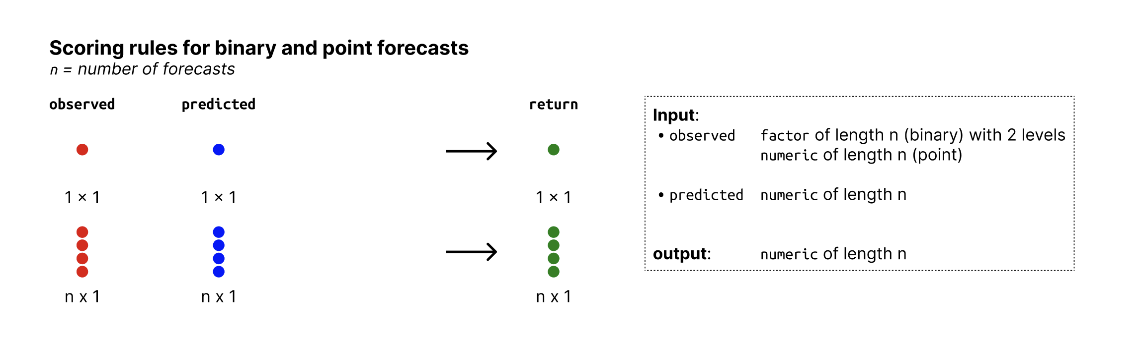
Overview of required input format for binary and point forecasts

See Also

Other get_metrics functions: get_metrics(), get_metrics.forecast_nominal(), get_metrics.forecast_ordinal(), get_metrics.forecast_point(), get_metrics.forecast_quantile(), get_metrics.forecast_sample(), get_metrics.scores()

Examples

get_metrics(example_binary)
get_metrics(example_binary, select = "brier_score")
get_metrics(example_binary, exclude = "log_score")

Get default metrics for nominal forecasts

Description

For nominal forecasts, the default scoring rule is:

• "log_score" = logs_categorical()

Usage

## S3 method for class 'forecast_nominal'
get_metrics(x, select = NULL, exclude = NULL, ...)

Arguments

See Also

Other get_metrics functions: get_metrics(), get_metrics.forecast_binary(), get_metrics.forecast_ordinal(), get_metrics.forecast_point(), get_metrics.forecast_quantile(), get_metrics.forecast_sample(), get_metrics.scores()

Examples

get_metrics(example_nominal)

Get default metrics for nominal forecasts

Description

For ordinal forecasts, the default scoring rules are:

• "log_score" = logs_categorical()

• "rps" = rps_ordinal()

Usage

## S3 method for class 'forecast_ordinal'
get_metrics(x, select = NULL, exclude = NULL, ...)

Arguments

See Also

Other get_metrics functions: get_metrics(), get_metrics.forecast_binary(), get_metrics.forecast_nominal(), get_metrics.forecast_point(), get_metrics.forecast_quantile(), get_metrics.forecast_sample(), get_metrics.scores()

Examples

get_metrics(example_ordinal)

Get default metrics for point forecasts

Description

For point forecasts, the default scoring rules are:

• "ae_point" = ae()

• "se_point" = se()

• "ape" = ape()

A note of caution: Every scoring rule for a point forecast is implicitly minimised by a specific aspect of the predictive distribution (see Gneiting, 2011).

The mean squared error, for example, is only a meaningful scoring rule if the forecaster actually reported the mean of their predictive distribution as a point forecast. If the forecaster reported the median, then the mean absolute error would be the appropriate scoring rule. If the scoring rule and the predictive task do not align, the results will be misleading.

Failure to respect this correspondence can lead to grossly misleading results! Consider the example in the section below.

Usage

## S3 method for class 'forecast_point'
get_metrics(x, select = NULL, exclude = NULL, ...)

Arguments

Input format

Overview of required input format for binary and point forecasts

References

Making and Evaluating Point Forecasts, Gneiting, Tilmann, 2011, Journal of the American Statistical Association.

See Also

Other get_metrics functions: get_metrics(), get_metrics.forecast_binary(), get_metrics.forecast_nominal(), get_metrics.forecast_ordinal(), get_metrics.forecast_quantile(), get_metrics.forecast_sample(), get_metrics.scores()

Examples

get_metrics(example_point, select = "ape")

library(magrittr)
set.seed(123)
n <- 500
observed <- rnorm(n, 5, 4)^2

predicted_mu <- mean(observed)
predicted_not_mu <- predicted_mu - rnorm(n, 10, 2)

df <- data.frame(
  model = rep(c("perfect", "bad"), each = n),
  predicted = c(rep(predicted_mu, n), predicted_not_mu),
  observed = rep(observed, 2),
  id = rep(1:n, 2)
) %>%
  as_forecast_point()
score(df) %>%
  summarise_scores()

Get default metrics for quantile-based forecasts

Description

For quantile-based forecasts, the default scoring rules are:

• "wis" = wis()

• "overprediction" = overprediction_quantile()

• "underprediction" = underprediction_quantile()

• "dispersion" = dispersion_quantile()

• "bias" = bias_quantile()

• "interval_coverage_50" = interval_coverage()

• "interval_coverage_90" = purrr::partial( interval_coverage, interval_range = 90 )

• "ae_median" = ae_median_quantile()

Note: The interval_coverage_90 scoring rule is created by modifying interval_coverage(), making use of the function purrr::partial(). This construct allows the function to deal with arbitrary arguments in ..., while making sure that only those that interval_coverage() can accept get passed on to it. interval_range = 90 is set in the function definition, as passing an argument interval_range = 90 to score() would mean it would also get passed to interval_coverage_50.

Usage

## S3 method for class 'forecast_quantile'
get_metrics(x, select = NULL, exclude = NULL, ...)

Arguments

Input format

Overview of required input format for quantile-based forecasts

See Also

Other get_metrics functions: get_metrics(), get_metrics.forecast_binary(), get_metrics.forecast_nominal(), get_metrics.forecast_ordinal(), get_metrics.forecast_point(), get_metrics.forecast_sample(), get_metrics.scores()

Examples

get_metrics(example_quantile, select = "wis")

Get default metrics for sample-based forecasts

Description

For sample-based forecasts, the default scoring rules are:

• "crps" = crps_sample()

• "overprediction" = overprediction_sample()

• "underprediction" = underprediction_sample()

• "dispersion" = dispersion_sample()

• "log_score" = logs_sample()

• "dss" = dss_sample()

• "mad" = mad_sample()

• "bias" = bias_sample()

• "ae_median" = ae_median_sample()

• "se_mean" = se_mean_sample()

Usage

## S3 method for class 'forecast_sample'
get_metrics(x, select = NULL, exclude = NULL, ...)

Arguments

Input format

Overview of required input format for sample-based forecasts

See Also

Other get_metrics functions: get_metrics(), get_metrics.forecast_binary(), get_metrics.forecast_nominal(), get_metrics.forecast_ordinal(), get_metrics.forecast_point(), get_metrics.forecast_quantile(), get_metrics.scores()

Examples

get_metrics(example_sample_continuous, exclude = "mad")

Get names of the metrics that were used for scoring

Description

When applying a scoring rule via score(), the names of the scoring rules become column names of the resulting data.table. In addition, an attribute metrics will be added to the output, holding the names of the scores as a vector.

This is done so that functions like get_forecast_unit() or summarise_scores() can still identify which columns are part of the forecast unit and which hold a score.

get_metrics() accesses and returns the metrics attribute. If there is no attribute, the function will return NULL (or, if error = TRUE will produce an error instead). In addition, it checks the column names of the input for consistency with the data stored in the metrics attribute.

Handling a missing or inconsistent metrics attribute:

If the metrics attribute is missing or is not consistent with the column names of the data.table, you can either

• run score() again, specifying names for the scoring rules manually, or

• add/update the attribute manually using attr(scores, "metrics") <- c("names", "of", "your", "scores") (the order does not matter).

Usage

## S3 method for class 'scores'
get_metrics(x, error = FALSE, ...)

Arguments

Value

Character vector with the names of the scoring rules that were used for scoring.

See Also

Other get_metrics functions: get_metrics(), get_metrics.forecast_binary(), get_metrics.forecast_nominal(), get_metrics.forecast_ordinal(), get_metrics.forecast_point(), get_metrics.forecast_quantile(), get_metrics.forecast_sample()

Obtain pairwise comparisons between models

Description

Compare scores obtained by different models in a pairwise tournament. All combinations of two models are compared against each other based on the overlapping set of available forecasts common to both models.

The input should be a scores object as produced by score(). Note that adding additional unrelated columns can unpredictably change results, as all present columns are taken into account when determining the set of overlapping forecasts between two models.

The output of the pairwise comparisons is a set of mean score ratios, relative skill scores and p-values.

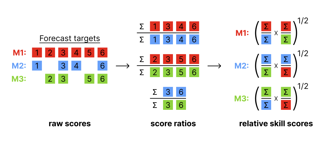
Illustration of the pairwise comparison process.

Mean score ratios

For every pair of two models, a mean score ratio is computed. This is simply the mean score of the first model divided by the mean score of the second. Mean score ratios are computed based on the set of overlapping forecasts between the two models. That means that only scores for those targets are taken into account for which both models have submitted a forecast.

(Scaled) Relative skill scores

The relative score of a model is the geometric mean of all mean score ratios which involve that model. If a baseline is provided, scaled relative skill scores will be calculated as well. Scaled relative skill scores are simply the relative skill score of a model divided by the relative skill score of the baseline model.

p-values

In addition, the function computes p-values for the comparison between two models (again based on the set of overlapping forecasts). P-values can be computed in two ways: based on a nonparametric Wilcoxon signed-rank test (internally using wilcox.test() with paired = TRUE) or based on a permutation test. The permutation test is based on the difference in mean scores between two models. The default null hypothesis is that the mean score difference is zero (see permutation_test()). Adjusted p-values are computed by calling p.adjust() on the raw p-values.

The code for the pairwise comparisons is inspired by an implementation by Johannes Bracher. The implementation of the permutation test follows the function permutationTest from the surveillance package by Michael Höhle, Andrea Riebler and Michaela Paul.

Usage

get_pairwise_comparisons(
  scores,
  compare = "model",
  by = NULL,
  metric = intersect(c("wis", "crps", "brier_score"), names(scores)),
  baseline = NULL,
  ...
)

Arguments

Value

A data.table with the results of pairwise comparisons containing the mean score ratios (mean_scores_ratio), unadjusted (pval) and adjusted (adj_pval) p-values, and relative skill values of each model (..._relative_skill). If a baseline model is given then the scaled relative skill is reported as well (..._scaled_relative_skill).

Author(s)

Nikos Bosse nikosbosse@gmail.com

Johannes Bracher, johannes.bracher@kit.edu

Examples

library(magrittr) # pipe operator

scores <- example_quantile %>%
 as_forecast_quantile() %>%
 score()

pairwise <- get_pairwise_comparisons(scores, by = "target_type")
pairwise2 <- get_pairwise_comparisons(
  scores, by = "target_type", baseline = "EuroCOVIDhub-baseline"
)

library(ggplot2)
plot_pairwise_comparisons(pairwise, type = "mean_scores_ratio") +
  facet_wrap(~target_type)

Probability integral transformation histogram

Description

Generate a Probability Integral Transformation (PIT) histogram for validated forecast objects.

See the examples for how to plot the result of this function.

Usage

## S3 method for class 'forecast_quantile'
get_pit_histogram(forecast, num_bins = NULL, breaks = NULL, by, ...)

## S3 method for class 'forecast_sample'
get_pit_histogram(
  forecast,
  num_bins = 10,
  breaks = NULL,
  by,
  integers = c("nonrandom", "random", "ignore"),
  n_replicates = NULL,
  ...
)

get_pit_histogram(forecast, num_bins, breaks, by, ...)

## Default S3 method:
get_pit_histogram(forecast, num_bins, breaks, by, ...)

Arguments

Value

A data.table with density values for each bin in the PIT histogram.

References

Sebastian Funk, Anton Camacho, Adam J. Kucharski, Rachel Lowe, Rosalind M. Eggo, W. John Edmunds (2019) Assessing the performance of real-time epidemic forecasts: A case study of Ebola in the Western Area region of Sierra Leone, 2014-15, doi:10.1371/journal.pcbi.1006785

See Also

pit_histogram_sample()

Examples

library("ggplot2")

result <- get_pit_histogram(example_sample_continuous, by = "model")
ggplot(result,  aes(x = mid, y = density)) +
  geom_col() +
  facet_wrap(. ~ model) +
  labs(x = "Quantile", "Density")

# example with quantile data
result <- get_pit_histogram(example_quantile, by = "model")
ggplot(result,  aes(x = mid, y = density)) +
  geom_col() +
  facet_wrap(. ~ model) +
  labs(x = "Quantile", "Density")

Get protected columns from data

Description

Helper function to get the names of all columns in a data frame that are protected columns.

Usage

get_protected_columns(data = NULL)

Arguments

Value

A character vector with the names of protected columns in the data. If data is NULL (default) then it returns a list of all columns that are protected in scoringutils.

Get interval range belonging to a quantile

Description

Every quantile can be thought of either as the lower or the upper bound of a symmetric central prediction interval. This helper function returns the range of the central prediction interval to which the quantile belongs.

Due to numeric instability that sometimes occurred in the past, ranges are rounded to 10 decimal places. This is not a problem for the vast majority of use cases, but it is something to be aware of.

Usage

get_range_from_quantile(quantile_level)

Arguments

Value

a numeric vector of interval ranges of size N

Get type of a vector or matrix of observed values or predictions

Description

Internal helper function to get the type of a vector (usually of observed or predicted values). The function checks whether the input is a factor, or else whether it is integer (or can be coerced to integer) or whether it's continuous.

Usage

get_type(x)

Arguments

Value

Character vector of length one with either "classification", "integer", or "continuous".

Illustration of required inputs for binary and point forecasts

Description

Illustration of required inputs for binary and point forecasts

Input format

Overview of required input format for binary and point forecasts

Illustration of required inputs for nominal forecasts

Description

Illustration of required inputs for nominal forecasts

Input format

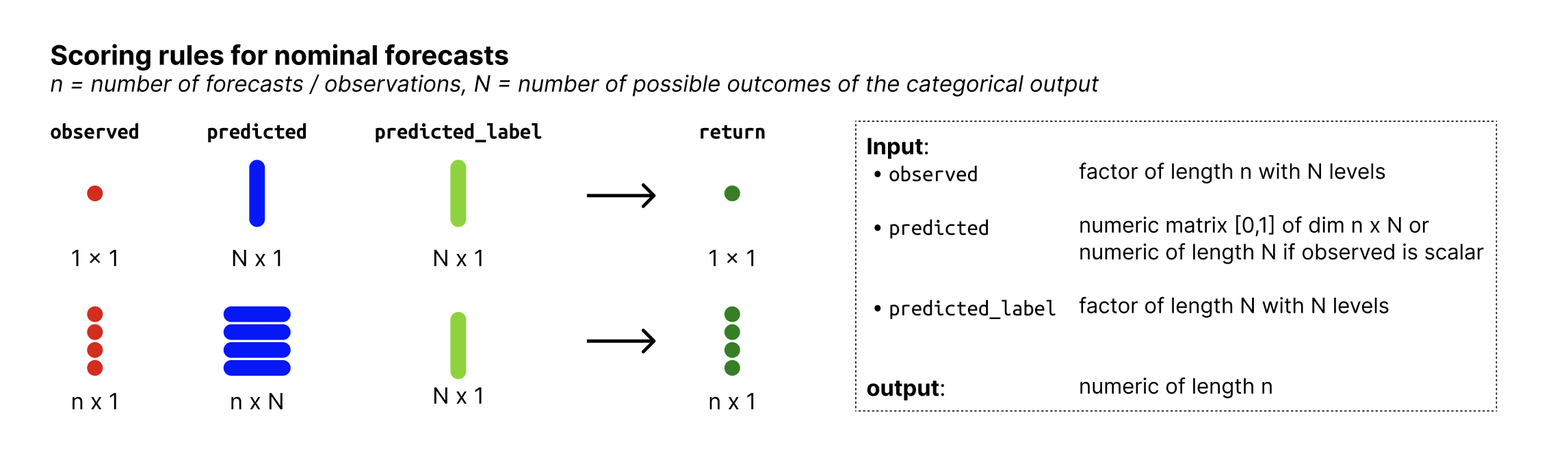
Overview of required input format for nominal forecasts

Illustration of required inputs for ordinal forecasts

Description

Illustration of required inputs for ordinal forecasts

Input format

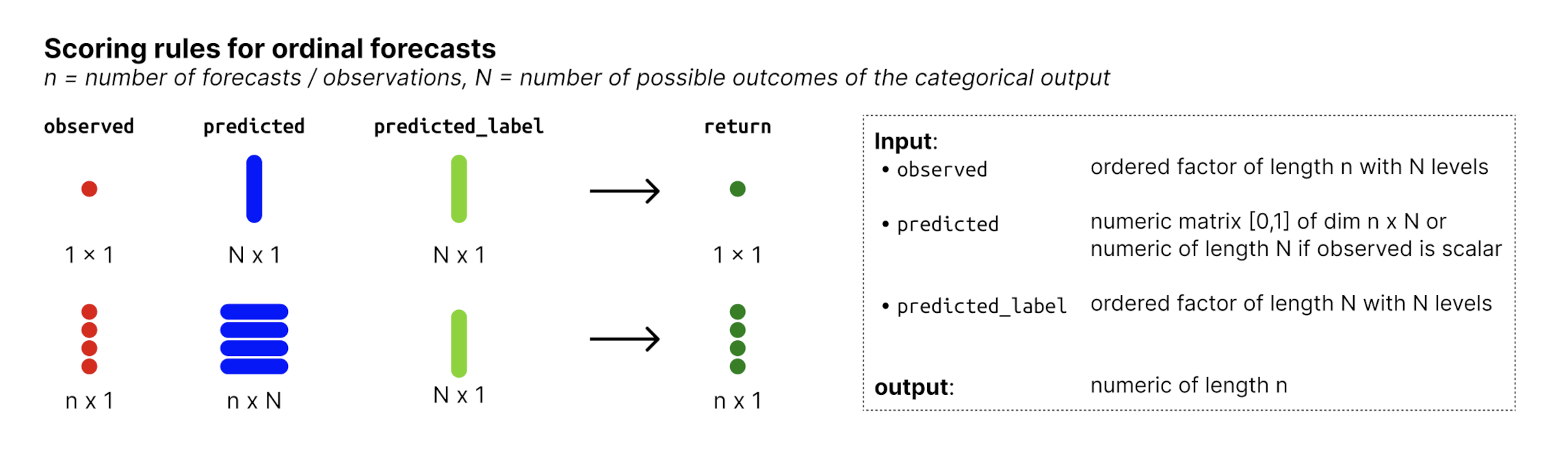
Overview of required input format for ordinal forecasts

Illustration of required inputs for quantile-based forecasts

Description

Illustration of required inputs for quantile-based forecasts

Input format

Overview of required input format for quantile-based forecasts

Illustration of required inputs for sample-based forecasts

Description

Illustration of required inputs for sample-based forecasts

Input format

Overview of required input format for sample-based forecasts

Helper function to interpolate the median prediction if it is not available

Description

Internal function to interpolate the median prediction if it is not available in the given quantile levels. This is done using linear interpolation between the two innermost quantiles.

Usage

interpolate_median(predicted, quantile_level)

Arguments

Value

scalar with the imputed median prediction

Input format

Overview of required input format for quantile-based forecasts

Interval coverage (for quantile-based forecasts)

Description

Check whether the observed value is within a given central prediction interval. The prediction interval is defined by a lower and an upper bound formed by a pair of predictive quantiles. For example, a 50% prediction interval is formed by the 0.25 and 0.75 quantiles of the predictive distribution.

Usage

interval_coverage(observed, predicted, quantile_level, interval_range = 50)

Arguments

Value

A vector of length n with elements either TRUE, if the observed value is within the corresponding prediction interval, and FALSE otherwise.

Input format

Overview of required input format for quantile-based forecasts

Examples

observed <- c(1, -15, 22)
predicted <- rbind(
  c(-1, 0, 1, 2, 3),
  c(-2, 1, 2, 2, 4),
   c(-2, 0, 3, 3, 4)
)
quantile_level <- c(0.1, 0.25, 0.5, 0.75, 0.9)
interval_coverage(observed, predicted, quantile_level)

Interval score

Description

Proper Scoring Rule to score quantile predictions, following Gneiting and Raftery (2007). Smaller values are better.

The score is computed as

\textrm{score} = (\textrm{upper} - \textrm{lower}) + \frac{2}{\alpha}(\textrm{lower} - \textrm{observed}) * \mathbf{1}(\textrm{observed} < \textrm{lower}) + \frac{2}{\alpha}(\textrm{observed} - \textrm{upper}) * \mathbf{1}(\textrm{observed} > \textrm{upper})

where \mathbf{1}() is the indicator function and indicates how much is outside the prediction interval. \alpha is the decimal value that indicates how much is outside the prediction interval.

To improve usability, the user is asked to provide an interval range in percentage terms, i.e. interval_range = 90 (percent) for a 90 percent prediction interval. Correspondingly, the user would have to provide the 5% and 95% quantiles (the corresponding alpha would then be 0.1). No specific distribution is assumed, but the interval has to be symmetric around the median (i.e you can't use the 0.1 quantile as the lower bound and the 0.7 quantile as the upper bound). Non-symmetric quantiles can be scored using the function quantile_score().

Usage

interval_score(
  observed,
  lower,
  upper,
  interval_range,
  weigh = TRUE,
  separate_results = FALSE
)

Arguments

Value

Vector with the scoring values, or a list with separate entries if separate_results is TRUE.

References

Strictly Proper Scoring Rules, Prediction,and Estimation, Tilmann Gneiting and Adrian E. Raftery, 2007, Journal of the American Statistical Association, Volume 102, 2007 - Issue 477

Evaluating epidemic forecasts in an interval format, Johannes Bracher, Evan L. Ray, Tilmann Gneiting and Nicholas G. Reich, https://journals.plos.org/ploscompbiol/article?id=10.1371/journal.pcbi.1008618 # nolint

Examples

observed <- rnorm(30, mean = 1:30)
interval_range <- rep(90, 30)
alpha <- (100 - interval_range) / 100
lower <- qnorm(alpha / 2, rnorm(30, mean = 1:30))
upper <- qnorm((1 - alpha / 2), rnorm(30, mean = 11:40))

scoringutils:::interval_score(
  observed = observed,
  lower = lower,
  upper = upper,
  interval_range = interval_range
)

# gives a warning, as the interval_range should likely be 50 instead of 0.5
scoringutils:::interval_score(
  observed = 4, upper = 8, lower = 2, interval_range = 0.5
)

# example with missing values and separate results
scoringutils:::interval_score(
  observed = c(observed, NA),
  lower = c(lower, NA),
  upper = c(NA, upper),
  separate_results = TRUE,
  interval_range = 90
)

Test whether an object is a forecast object

Description

Test whether an object is a forecast object.

You can test for a specific ⁠forecast_<type>⁠ class using the appropriate ⁠is_forecast_<type>⁠ function.

Usage

is_forecast_binary(x)

is_forecast_nominal(x)

is_forecast_ordinal(x)

is_forecast_point(x)

is_forecast_quantile(x)

is_forecast_sample(x)

is_forecast(x)

Arguments

Value

is_forecast: TRUE if the object is of class forecast, FALSE otherwise.

⁠is_forecast_<type>*⁠: TRUE if the object is of class ⁠forecast_*⁠ in addition to class forecast, FALSE otherwise.

Examples

forecast_binary <- as_forecast_binary(example_binary)
is_forecast(forecast_binary)

Log transformation with an additive shift

Description

Function that shifts a value by some offset and then applies the natural logarithm to it.

Usage

log_shift(x, offset = 0, base = exp(1))

Arguments

Details

The output is computed as log(x + offset)

Value

A numeric vector with transformed values

References

Transformation of forecasts for evaluating predictive performance in an epidemiological context Nikos I. Bosse, Sam Abbott, Anne Cori, Edwin van Leeuwen, Johannes Bracher, Sebastian Funk medRxiv 2023.01.23.23284722 doi:10.1101/2023.01.23.23284722 https://www.medrxiv.org/content/10.1101/2023.01.23.23284722v1 # nolint

Examples

library(magrittr) # pipe operator
log_shift(1:10)
log_shift(0:9, offset = 1)

example_quantile[observed > 0, ] %>%
  as_forecast_quantile() %>%
  transform_forecasts(fun = log_shift, offset = 1)

Log score for categorical outcomes

Description

Log score for categorical (nominal or ordinal) outcomes

The Log Score is the negative logarithm of the probability assigned to the observed value. It is a proper scoring rule. Small values are better (best is zero, worst is infinity).

Usage

logs_categorical(observed, predicted, predicted_label)

Arguments

Value

A numeric vector of size n with log scores

Input format

Overview of required input format for nominal forecasts

See Also

Other log score functions: logs_sample(), scoring-functions-binary

Examples

factor_levels <- c("one", "two", "three")
predicted_label <- factor(c("one", "two", "three"), levels = factor_levels)
observed <- factor(c("one", "three", "two"), levels = factor_levels)
predicted <- matrix(
  c(0.8, 0.1, 0.1,
    0.1, 0.2, 0.7,
    0.4, 0.4, 0.2),
  nrow = 3,
  byrow = TRUE
)
logs_categorical(observed, predicted, predicted_label)

Logarithmic score (sample-based version)

Description

This function is a wrapper around the logs_sample() function from the scoringRules package.

The log score is the negative logarithm of the predictive density evaluated at the observed value.

The function should be used to score continuous predictions only. While the Log Score is in theory also applicable to discrete forecasts, the problem lies in the implementation: The function uses a kernel density estimation, which is not well defined with integer-valued Monte Carlo Samples. See the scoringRules package for more details and alternatives, e.g. calculating scores for specific discrete probability distributions.

Usage

logs_sample(observed, predicted, ...)

Arguments

Value

Vector with scores.

Input format

Overview of required input format for sample-based forecasts

References

Alexander Jordan, Fabian Krüger, Sebastian Lerch, Evaluating Probabilistic Forecasts with scoringRules, https://www.jstatsoft.org/article/view/v090i12

See Also

Other log score functions: logs_categorical(), scoring-functions-binary

Examples

observed <- rpois(30, lambda = 1:30)
predicted <- replicate(200, rpois(n = 30, lambda = 1:30))
logs_sample(observed, predicted)

Determine dispersion of a probabilistic forecast

Description

Sharpness is the ability of the model to generate predictions within a narrow range and dispersion is the lack thereof. It is a data-independent measure, and is purely a feature of the forecasts themselves.

Dispersion of predictive samples corresponding to one single observed value is measured as the normalised median of the absolute deviation from the median of the predictive samples. For details, see mad() and the explanations given in Funk et al. (2019)

Usage

mad_sample(observed = NULL, predicted, ...)

Arguments

Value

Vector with dispersion values.

Input format

Overview of required input format for sample-based forecasts

References

Funk S, Camacho A, Kucharski AJ, Lowe R, Eggo RM, Edmunds WJ (2019) Assessing the performance of real-time epidemic forecasts: A case study of Ebola in the Western Area region of Sierra Leone, 2014-15. PLoS Comput Biol 15(2): e1006785. doi:10.1371/journal.pcbi.1006785

Examples

predicted <- replicate(200, rpois(n = 30, lambda = 1:30))
mad_sample(predicted = predicted)

Class constructor for forecast objects

Description

Construct a class based on a data.frame or similar. The constructor

• coerces the data into a data.table

• assigns a class

Usage

new_forecast(data, classname)

Arguments

Value

An object of the class indicated by classname

Construct an object of class scores

Description

This function creates an object of class scores based on a data.table or similar.

Usage

new_scores(scores, metrics, ...)

Arguments

Value

An object of class scores

Examples

## Not run: 
df <- data.frame(
  model = "A",
  wis = "0.1"
)
new_scores(df, "wis")

## End(Not run)

Do pairwise comparison for one set of forecasts

Description

This function does the pairwise comparison for one set of forecasts, but multiple models involved. It gets called from get_pairwise_comparisons(). get_pairwise_comparisons() splits the data into arbitrary subgroups specified by the user (e.g. if pairwise comparison should be done separately for different forecast targets) and then the actual pairwise comparison for that subgroup is managed from pairwise_comparison_one_group(). In order to actually do the comparison between two models over a subset of common forecasts it calls compare_forecasts().

Usage

pairwise_comparison_one_group(
  scores,
  metric,
  baseline,
  compare = "model",
  by,
  ...
)

Arguments

Value

A data.table with the results of pairwise comparisons containing the mean score ratios (mean_scores_ratio), unadjusted (pval) and adjusted (adj_pval) p-values, and relative skill values of each model (..._relative_skill). If a baseline model is given then the scaled relative skill is reported as well (..._scaled_relative_skill).

Simple permutation test

Description

The implementation of the permutation test follows the function permutationTest from the surveillance package by Michael Höhle, Andrea Riebler and Michaela Paul. The function compares two vectors of scores. It computes the mean of each vector independently and then takes either the difference or the ratio of the two. This observed difference or ratio is compared against the same test statistic based on permutations of the original data.

Used in get_pairwise_comparisons().

Usage

permutation_test(
  scores1,
  scores2,
  n_permutation = 999,
  one_sided = FALSE,
  comparison_mode = c("difference", "ratio")
)

Arguments

Value

p-value of the permutation test

Probability integral transformation for counts

Description

Uses a Probability integral transformation (PIT) (or a randomised PIT for integer forecasts) to assess the calibration of predictive Monte Carlo samples.

Usage

pit_histogram_sample(
  observed,
  predicted,
  quantiles,
  integers = c("nonrandom", "random", "ignore"),
  n_replicates = NULL
)

Arguments

Details

Calibration or reliability of forecasts is the ability of a model to correctly identify its own uncertainty in making predictions. In a model with perfect calibration, the observed data at each time point look as if they came from the predictive probability distribution at that time.

Equivalently, one can inspect the probability integral transform of the predictive distribution at time t,

u_t = F_t (x_t)

where x_t is the observed data point at time t \textrm{ in } t_1, …, t_n, n being the number of forecasts, and F_t is the (continuous) predictive cumulative probability distribution at time t. If the true probability distribution of outcomes at time t is G_t then the forecasts F_t are said to be ideal if F_t = G_t at all times t. In that case, the probabilities u_t are distributed uniformly.

In the case of discrete nonnegative outcomes such as incidence counts, the PIT is no longer uniform even when forecasts are ideal. In that case two methods are available ase described by Czado et al. (2007).

By default, a nonrandomised PIT is calculated using the conditional cumulative distribution function

F(u) = \begin{cases} 0 & \text{if } v < P_t(k_t - 1) \\ (v - P_t(k_t - 1)) / (P_t(k_t) - P_t(k_t - 1)) & \text{if } P_t(k_t - 1) \leq v < P_t(k_t) \\ 1 & \text{if } v \geq P_t(k_t) \end{cases}

where k_t is the observed count, P_t(x) is the predictive cumulative probability of observing incidence k at time t and P_t (-1) = 0 by definition. Values of the PIT histogram are then created by averaging over the n predictions,

\bar{F}(u) = \frac{i = 1}{n} \sum_{i=1}^{n} F^{(i)}(u)

And calculating the value at each bin between quantile q_i and quantile q_{i + 1} as

\bar{F}(q_i) - \bar{F}(q_{i + 1})

Alternatively, a randomised PIT can be used instead. In this case, the PIT is

u_t = P_t(k_t) + v * (P_t(k_t) - P_t(k_t - 1))

where v is standard uniform and independent of k. The values of the PIT histogram are then calculated by binning the u_t values as above.

Value

A vector with PIT histogram densities for the bins corresponding to the given quantiles.

References

Claudia Czado, Tilmann Gneiting Leonhard Held (2009) Predictive model assessment for count data. Biometrika, 96(4), 633-648. Sebastian Funk, Anton Camacho, Adam J. Kucharski, Rachel Lowe, Rosalind M. Eggo, W. John Edmunds (2019) Assessing the performance of real-time epidemic forecasts: A case study of Ebola in the Western Area region of Sierra Leone, 2014-15, doi:10.1371/journal.pcbi.1006785

See Also

get_pit_histogram()

Examples

## continuous predictions
observed <- rnorm(20, mean = 1:20)
predicted <- replicate(100, rnorm(n = 20, mean = 1:20))
pit <- pit_histogram_sample(observed, predicted, quantiles = seq(0, 1, 0.1))

## integer predictions
observed <- rpois(20, lambda = 1:20)
predicted <- replicate(100, rpois(n = 20, lambda = 1:20))
pit <- pit_histogram_sample(observed, predicted, quantiles = seq(0, 1, 0.1))

## integer predictions, randomised PIT
observed <- rpois(20, lambda = 1:20)
predicted <- replicate(100, rpois(n = 20, lambda = 1:20))
pit <- pit_histogram_sample(
  observed, predicted, quantiles = seq(0, 1, 0.1),
  integers = "random", n_replicates = 30
)

Plot correlation between metrics

Description

Plots a heatmap of correlations between different metrics.

Usage

plot_correlations(correlations, digits = NULL)

Arguments

Value

A ggplot object showing a coloured matrix of correlations between metrics.

A ggplot object with a visualisation of correlations between metrics

Examples

library(magrittr) # pipe operator
scores <- example_quantile %>%
  as_forecast_quantile %>%
  score()
correlations <- scores %>%
  summarise_scores() %>%
  get_correlations()
plot_correlations(correlations, digits = 2)

Visualise the number of available forecasts

Description

Visualise Where Forecasts Are Available.

Usage

plot_forecast_counts(
  forecast_counts,
  x,
  y = "model",
  x_as_factor = TRUE,
  show_counts = TRUE
)

Arguments

Value

A ggplot object with a plot of forecast counts

Examples

library(ggplot2)
library(magrittr) # pipe operator
forecast_counts <- example_quantile %>%
  as_forecast_quantile %>%
  get_forecast_counts(by = c("model", "target_type", "target_end_date"))
plot_forecast_counts(
 forecast_counts, x = "target_end_date", show_counts = FALSE
) +
 facet_wrap("target_type")

Create a heatmap of a scoring metric

Description

This function can be used to create a heatmap of one metric across different groups, e.g. the interval score obtained by several forecasting models in different locations.

Usage

plot_heatmap(scores, y = "model", x, metric)

Arguments

Value

A ggplot object showing a heatmap of the desired metric

Examples

library(magrittr) # pipe operator
scores <- example_quantile %>%
  as_forecast_quantile %>%
  score()
scores <- summarise_scores(scores, by = c("model", "target_type"))
scores <- summarise_scores(
  scores, by = c("model", "target_type"),
  fun = signif, digits = 2
)

plot_heatmap(scores, x = "target_type", metric = "bias")

Plot interval coverage

Description

Plot interval coverage values (see get_coverage() for more information).

Usage

plot_interval_coverage(coverage, colour = "model")

Arguments

Value

ggplot object with a plot of interval coverage

Examples

example <- as_forecast_quantile(example_quantile)
coverage <- get_coverage(example, by = "model")
plot_interval_coverage(coverage)

Plot heatmap of pairwise comparisons

Description

Creates a heatmap of the ratios or pvalues from a pairwise comparison between models.

Usage

plot_pairwise_comparisons(
  comparison_result,
  type = c("mean_scores_ratio", "pval")
)

Arguments

Value

A ggplot object with a heatmap of mean score ratios from pairwise comparisons.

Examples

library(ggplot2)
library(magrittr) # pipe operator
scores <- example_quantile %>%
  as_forecast_quantile %>%
  score()
pairwise <- get_pairwise_comparisons(scores, by = "target_type")
plot_pairwise_comparisons(pairwise, type = "mean_scores_ratio") +
  facet_wrap(~target_type)

Plot quantile coverage

Description

Plot quantile coverage values (see get_coverage() for more information).

Usage

plot_quantile_coverage(coverage, colour = "model")

Arguments

Value

A ggplot object with a plot of interval coverage

Examples

example <- as_forecast_quantile(example_quantile)
coverage <- get_coverage(example, by = "model")
plot_quantile_coverage(coverage)

Plot contributions to the weighted interval score

Description

Visualise the components of the weighted interval score: penalties for over-prediction, under-prediction and for high dispersion (lack of sharpness).

Usage

plot_wis(scores, x = "model", relative_contributions = FALSE, flip = FALSE)

Arguments

Value

A ggplot object showing a contributions from the three components of the weighted interval score.

A ggplot object with a visualisation of the WIS decomposition

References

Bracher J, Ray E, Gneiting T, Reich, N (2020) Evaluating epidemic forecasts in an interval format. https://journals.plos.org/ploscompbiol/article?id=10.1371/journal.pcbi.1008618

Examples

library(ggplot2)
library(magrittr) # pipe operator
scores <- example_quantile %>%
  as_forecast_quantile %>%
  score()
scores <- summarise_scores(scores, by = c("model", "target_type"))

plot_wis(scores,
  x = "model",
  relative_contributions = TRUE
) +
  facet_wrap(~target_type)
plot_wis(scores,
  x = "model",
  relative_contributions = FALSE
) +
  facet_wrap(~target_type, scales = "free_x")

Print information about a forecast object

Description

This function prints information about a forecast object, including "Forecast type", "Score columns", "Forecast unit".

Usage

## S3 method for class 'forecast'
print(x, ...)

Arguments

Value

Returns x invisibly.

Examples

dat <- as_forecast_quantile(example_quantile)
print(dat)

Quantile score

Description

Proper Scoring Rule to score quantile predictions. Smaller values are better. The quantile score is closely related to the interval score (see wis()) and is the quantile equivalent that works with single quantiles instead of central prediction intervals.

The quantile score, also called pinball loss, for a single quantile level \tau is defined as

\text{QS}_\tau(F, y) = 2 \cdot \{ \mathbf{1}(y \leq q_\tau) - \tau\} \cdot (q_\tau - y) = \begin{cases} 2 \cdot (1 - \tau) * q_\tau - y, & \text{if } y \leq q_\tau\\ 2 \cdot \tau * |q_\tau - y|, & \text{if } y > q_\tau, \end{cases}

with q_\tau being the \tau-quantile of the predictive distribution F, and \mathbf{1}(\cdot) the indicator function.

The weighted interval score for a single prediction interval can be obtained as the average of the quantile scores for the lower and upper quantile of that prediction interval:

\text{WIS}_\alpha(F, y) = \frac{\text{QS}_{\alpha/2}(F, y) + \text{QS}_{1 - \alpha/2}(F, y)}{2}.

See the SI of Bracher et al. (2021) for more details.

quantile_score() returns the average quantile score across the quantile levels provided. For a set of quantile levels that form pairwise central prediction intervals, the quantile score is equivalent to the interval score.

Usage

quantile_score(observed, predicted, quantile_level, weigh = TRUE)

Arguments

Value

Numeric vector of length n with the quantile score. The scores are averaged across quantile levels if multiple quantile levels are provided (the result of calling rowMeans() on the matrix of quantile scores that is computed based on the observed and predicted values).

Input format

Overview of required input format for quantile-based forecasts

References

Strictly Proper Scoring Rules, Prediction,and Estimation, Tilmann Gneiting and Adrian E. Raftery, 2007, Journal of the American Statistical Association, Volume 102, 2007 - Issue 477

Evaluating epidemic forecasts in an interval format, Johannes Bracher, Evan L. Ray, Tilmann Gneiting and Nicholas G. Reich, 2021, https://journals.plos.org/ploscompbiol/article?id=10.1371/journal.pcbi.1008618

Examples

observed <- rnorm(10, mean = 1:10)
alpha <- 0.5

lower <- qnorm(alpha / 2, observed)
upper <- qnorm((1 - alpha / 2), observed)

qs_lower <- quantile_score(observed,
  predicted = matrix(lower),
  quantile_level = alpha / 2
)
qs_upper <- quantile_score(observed,
  predicted = matrix(upper),
  quantile_level = 1 - alpha / 2
)
interval_score <- (qs_lower + qs_upper) / 2
interval_score2 <- quantile_score(
  observed,
  predicted = cbind(lower, upper),
  quantile_level = c(alpha / 2, 1 - alpha / 2)
)

# this is the same as the following
wis(
  observed,
  predicted = cbind(lower, upper),
  quantile_level = c(alpha / 2, 1 - alpha / 2)
)

Transform from a quantile format to an interval format

Description

Internal helper function to transform from a quantile format to an interval format (which is no longer a supported forecast format, but still used internally. The function mimics an S3 generic, but is not actually an S3 generic, as we want the functions to be internal and not exported.)

Quantile format In a quantile format, a prediction is characterised by one or multiple predicted values and the corresponding quantile levels. For example, a prediction in a quantile format could be represented by the 0.05, 0.25, 0.5, 0.75 and 0.95 quantiles of the predictive distribution.

Interval format In the interval format, two quantiles are assumed to form a prediction interval. Prediction intervals need to be symmetric around the median and are characterised by a lower and an upper bound. The lower bound is defined by the lower quantile and the upper bound is defined by the upper quantile. A 90% prediction interval, for example, covers 90% of the probability mass and is defined by the 5% and 95% quantiles. A forecast could therefore be characterised by one or multiple prediction intervals, e.g. the lower and upper bounds of the 50% and 90% prediction intervals (corresponding to the 0.25 and 0.75 as well as the 0.05 and 0.095 quantiles).

Usage

quantile_to_interval(...)

quantile_to_interval_dataframe(
  forecast,
  format = "long",
  keep_quantile_col = FALSE,
  ...
)

quantile_to_interval_numeric(observed, predicted, quantile_level, ...)

Arguments

Value

A data.table with forecasts in an interval format.

quantile_to_interval_dataframe: a data.table in an interval format (either "long" or "wide"), with or without a quantile_level column. Rows will not be reordered.

quantile_to_interval.numeric: a data.table in a wide interval format with columns forecast_id, observed, lower, upper, and interval_range. The forecast_id column is a unique identifier for each forecast. Rows will be reordered according to forecast_id and interval_range.

Ranked Probability Score for ordinal outcomes

Description

The Ranked Probability Score (RPS) measures the difference between the predicted and observed cumulative distribution functions. It is a proper scoring rule that takes the ordering of categories into account. Small values are better (best is zero, worst is N - 1 where N is the number of categories).

Usage

rps_ordinal(observed, predicted, predicted_label)

Arguments

Value

A numeric vector of size n with ranked probability scores

Input format

Overview of required input format for nominal forecasts

Examples

factor_levels <- c("one", "two", "three")
predicted_label <- factor(factor_levels, levels = factor_levels, ordered = TRUE)
observed <- factor(c("three", "three", "two"), levels = factor_levels, ordered = TRUE)
predicted <- matrix(
  c(0.8, 0.1, 0.1,
    0.1, 0.2, 0.7,
    0.4, 0.4, 0.2),
  nrow = 3,
  byrow = TRUE
)
rps_ordinal(observed, predicted, predicted_label)

Run a function safely

Description

This is a wrapper/helper function designed to run a function safely when it is not completely clear what arguments could be passed to the function.

All named arguments in ... that are not accepted by fun are removed. All unnamed arguments are passed on to the function. In case fun errors, the error will be converted to a warning and run_safely returns NULL.

run_safely can be useful when constructing functions to be used as metrics in score().

Usage

run_safely(..., fun, metric_name)

Arguments

Value

The result of fun or NULL if fun errors

Examples

f <- function(x) {x}
scoringutils:::run_safely(2, fun = f, metric_name = "f")
scoringutils:::run_safely(2, y = 3, fun = f, metric_name = "f")
scoringutils:::run_safely(fun = f, metric_name = "f")
scoringutils:::run_safely(y = 3, fun = f, metric_name = "f")

Change data from a sample-based format to a long interval range format

Description

Transform data from a format that is based on predictive samples to a format based on interval ranges.

Usage

sample_to_interval_long(
  data,
  interval_range = c(0, 50, 90),
  type = 7,
  keep_quantile_col = TRUE
)

Arguments

Value

A data.table in a long interval interval range format

Evaluate forecasts

Description

score() applies a selection of scoring metrics to a forecast object. score() is a generic that dispatches to different methods depending on the class of the input data.

See as_forecast_binary(), as_forecast_quantile() etc. for information on how to create a forecast object.

See get_forecast_unit() for more information on the concept of a forecast unit.

For additional help and examples, check out the paper Evaluating Forecasts with scoringutils in R.

Usage

## S3 method for class 'forecast_binary'
score(forecast, metrics = get_metrics(forecast), ...)

## S3 method for class 'forecast_nominal'
score(forecast, metrics = get_metrics(forecast), ...)

## S3 method for class 'forecast_ordinal'
score(forecast, metrics = get_metrics(forecast), ...)

## S3 method for class 'forecast_point'
score(forecast, metrics = get_metrics(forecast), ...)

## S3 method for class 'forecast_quantile'
score(forecast, metrics = get_metrics(forecast), ...)

## S3 method for class 'forecast_sample'
score(forecast, metrics = get_metrics(forecast), ...)

score(forecast, metrics, ...)

Arguments

Details

Customising metrics

If you want to pass arguments to a scoring function, you need change the scoring function itself via e.g. purrr::partial() and pass an updated list of functions with your custom metric to the metrics argument in score(). For example, to use interval_coverage() with interval_range = 90, you would define a new function, e.g. interval_coverage_90 <- purrr::partial(interval_coverage, interval_range = 90) and pass this new function to metrics in score().

Note that if you want to pass a variable as an argument, you can unquote it with ⁠!!⁠ to make sure the value is evaluated only once when the function is created. Consider the following example:

custom_arg <- "foo"
print1 <- purrr::partial(print, x = custom_arg)
print2 <- purrr::partial(print, x = !!custom_arg)

custom_arg <- "bar"
print1() # prints 'bar'
print2() # prints 'foo'

Value

An object of class scores. This object is a data.table with unsummarised scores (one score per forecast) and has an additional attribute metrics with the names of the metrics used for scoring. See summarise_scores()) for information on how to summarise scores.

Author(s)

Nikos Bosse nikosbosse@gmail.com

References

Bosse NI, Gruson H, Cori A, van Leeuwen E, Funk S, Abbott S (2022) Evaluating Forecasts with scoringutils in R. doi:10.48550/arXiv.2205.07090

Examples

library(magrittr) # pipe operator


validated <- as_forecast_quantile(example_quantile)
score(validated) %>%
  summarise_scores(by = c("model", "target_type"))

# set forecast unit manually (to avoid issues with scoringutils trying to
# determine the forecast unit automatically)
example_quantile %>%
  as_forecast_quantile(
    forecast_unit = c(
      "location", "target_end_date", "target_type", "horizon", "model"
    )
  ) %>%
  score()

# forecast formats with different metrics
## Not run: 
score(as_forecast_binary(example_binary))
score(as_forecast_quantile(example_quantile))
score(as_forecast_point(example_point))
score(as_forecast_sample(example_sample_discrete))
score(as_forecast_sample(example_sample_continuous))

## End(Not run)

Metrics for binary outcomes

Description

Brier score

The Brier Score is the mean squared error between the probabilistic prediction and the observed outcome. The Brier score is a proper scoring rule. Small values are better (best is 0, the worst is 1).

\textrm{Brier\_Score} = (\textrm{prediction} - \textrm{outcome})^2,

where \textrm{outcome} \in \{0, 1\}, and \textrm{prediction} \in [0, 1] represents the probability that the outcome is equal to 1.

Log score for binary outcomes

The Log Score is the negative logarithm of the probability assigned to the observed value. It is a proper scoring rule. Small values are better (best is zero, worst is infinity).

Usage

brier_score(observed, predicted)

logs_binary(observed, predicted)

Arguments

Details

The functions require users to provide observed values as a factor in order to distinguish its input from the input format required for scoring point forecasts. Internally, however, factors will be converted to numeric values. A factor ⁠observed = factor(c(0, 1, 1, 0, 1)⁠ with two levels (0 and 1) would internally be coerced to a numeric vector (in this case this would result in the numeric vector c(1, 2, 2, 1, 1)). After subtracting 1, the resulting vector (c(0, 1, 1, 0) in this case) is used for internal calculations. All predictions are assumed represent the probability that the outcome is equal of the last/highest factor level (in this case that the outcome is equal to 1).

You could alternatively also provide a vector like observed = factor(c("a", "b", "b", "a")) (with two levels, a and b), which would result in exactly the same internal representation. Probabilities then represent the probability that the outcome is equal to "b". If you want your predictions to be probabilities that the outcome is "a", then you could of course make observed a factor with levels swapped, i.e. observed = factor(c("a", "b", "b", "a"), levels = c("b", "a"))

Value

A numeric vector of size n with the Brier scores

A numeric vector of size n with log scores

Input format

Overview of required input format for binary and point forecasts

See Also

Other log score functions: logs_categorical(), logs_sample()

Examples

observed <- factor(sample(c(0, 1), size = 30, replace = TRUE))
predicted <- runif(n = 30, min = 0, max = 1)

brier_score(observed, predicted)
logs_binary(observed, predicted)

Squared error of the mean (sample-based version)

Description

Squared error of the mean calculated as

\textrm{mean}(\textrm{observed} - \textrm{mean prediction})^2

The mean prediction is calculated as the mean of the predictive samples.

Usage

se_mean_sample(observed, predicted)

Arguments

Input format

Overview of required input format for sample-based forecasts

Examples

observed <- rnorm(30, mean = 1:30)
predicted_values <- matrix(rnorm(30, mean = 1:30))
se_mean_sample(observed, predicted_values)

Select metrics from a list of functions

Description

Helper function to return only the scoring rules selected by the user from a list of possible functions.

Usage

select_metrics(metrics, select = NULL, exclude = NULL)

Arguments

Value

A list of scoring functions.

Examples

select_metrics(
  metrics = get_metrics(example_binary),
  select = "brier_score"
)
select_metrics(
  metrics = get_metrics(example_binary),
  exclude = "log_score"
)

Set unit of a single forecast manually

Description

Helper function to set the unit of a single forecast (i.e. the combination of columns that uniquely define a single forecast) manually. This simple function keeps the columns specified in forecast_unit (plus additional protected columns, e.g. for observed values, predictions or quantile levels) and removes duplicate rows. set_forecast_unit() will mainly be called when constructing a forecast object via the forecast_unit argument in ⁠as_forecast_<type>⁠.

If not done explicitly, scoringutils attempts to determine the unit of a single forecast automatically by simply assuming that all column names are relevant to determine the forecast unit. This may lead to unexpected behaviour, so setting the forecast unit explicitly can help make the code easier to debug and easier to read.

Usage

set_forecast_unit(data, forecast_unit)

Arguments

Value

A data.table with only those columns kept that are relevant to scoring or denote the unit of a single forecast as specified by the user.

Examples

library(magrittr) # pipe operator
example_quantile %>%
  scoringutils:::set_forecast_unit(
    c("location", "target_end_date", "target_type", "horizon", "model")
  )

Summarise scores as produced by score()

Description

Summarise scores as produced by score().

summarise_scores relies on a way to identify the names of the scores and distinguish them from columns that denote the unit of a single forecast. Internally, this is done via a stored attribute, metrics that stores the names of the scores. This means, however, that you need to be careful with renaming scores after they have been produced by score(). If you do, you also have to manually update the attribute by calling attr(scores, "metrics") <- new_names.

Usage

summarise_scores(scores, by = "model", fun = mean, ...)

summarize_scores(scores, by = "model", fun = mean, ...)

Arguments

Value

A data.table with summarised scores. Scores are summarised according to the names of the columns of the original data specified in by using the fun passed to summarise_scores().

Examples

library(magrittr) # pipe operator
scores <- example_sample_continuous %>%
 as_forecast_sample() %>%
 score()

# get scores by model
summarise_scores(scores, by = "model")

# get scores by model and target type
summarise_scores(scores, by = c("model", "target_type"))

# get standard deviation
summarise_scores(scores, by = "model", fun = sd)

# round digits
summarise_scores(scores, by = "model") %>%
  summarise_scores(fun = signif, digits = 2)

Test whether column names are NOT present in a data.frame

Description

The function checks whether all column names are NOT present. If none of the columns are present, the function returns TRUE. If one or more columns are present, the function returns FALSE.

Usage

test_columns_not_present(data, columns)

Arguments

Value

Returns TRUE if none of the columns are present and FALSE otherwise

Test whether all column names are present in a data.frame

Description

The function checks whether all column names are present. If one or more columns are missing, the function returns FALSE. If all columns are present, the function returns TRUE.

Usage

test_columns_present(data, columns)

Arguments

Value

Returns TRUE if all columns are present and FALSE otherwise

Scoringutils ggplot2 theme

Description

A theme for ggplot2 plots used in scoringutils.

Usage

theme_scoringutils()

Value

A ggplot2 theme

Transform forecasts and observed values

Description

Function to transform forecasts and observed values before scoring.

Usage

transform_forecasts(
  forecast,
  fun = log_shift,
  append = TRUE,
  label = "log",
  ...
)

Arguments

Details

There are a few reasons, depending on the circumstances, for why this might be desirable (check out the linked reference for more info). In epidemiology, for example, it may be useful to log-transform incidence counts before evaluating forecasts using scores such as the weighted interval score (WIS) or the continuous ranked probability score (CRPS). Log-transforming forecasts and observations changes the interpretation of the score from a measure of absolute distance between forecast and observation to a score that evaluates a forecast of the exponential growth rate. Another motivation can be to apply a variance-stabilising transformation or to standardise incidence counts by population.

Note that if you want to apply a transformation, it is important to transform the forecasts and observations and then apply the score. Applying a transformation after the score risks losing propriety of the proper scoring rule.

Value

A forecast object with either a transformed version of the data, or one with both the untransformed and the transformed data. includes the original data as well as a transformation of the original data. There will be one additional column, ‘scale’, present which will be set to "natural" for the untransformed forecasts.

Author(s)

Nikos Bosse nikosbosse@gmail.com

References

Transformation of forecasts for evaluating predictive performance in an epidemiological context Nikos I. Bosse, Sam Abbott, Anne Cori, Edwin van Leeuwen, Johannes Bracher, Sebastian Funk medRxiv 2023.01.23.23284722 doi:10.1101/2023.01.23.23284722 https://www.medrxiv.org/content/10.1101/2023.01.23.23284722v1

Examples

library(magrittr) # pipe operator

# transform forecasts using the natural logarithm
# negative values need to be handled (here by replacing them with 0)
example_quantile %>%
  .[, observed := ifelse(observed < 0, 0, observed)] %>%
  as_forecast_quantile() %>%
# Here we use the default function log_shift() which is essentially the same
# as log(), but has an additional arguments (offset) that allows you add an
# offset before applying the logarithm.
  transform_forecasts(append = FALSE) %>%
  head()

# alternatively, integrating the truncation in the transformation function:
example_quantile %>%
  as_forecast_quantile() %>%
 transform_forecasts(
   fun = function(x) {log_shift(pmax(0, x))}, append = FALSE
 ) %>%
 head()

# specifying an offset for the log transformation removes the
# warning caused by zeros in the data
example_quantile %>%
  as_forecast_quantile() %>%
  .[, observed := ifelse(observed < 0, 0, observed)] %>%
  transform_forecasts(offset = 1, append = FALSE) %>%
  head()

# adding square root transformed forecasts to the original ones
example_quantile %>%
  .[, observed := ifelse(observed < 0, 0, observed)] %>%
  as_forecast_quantile() %>%
  transform_forecasts(fun = sqrt, label = "sqrt") %>%
  score() %>%
  summarise_scores(by = c("model", "scale"))

# adding multiple transformations
example_quantile %>%
  as_forecast_quantile() %>%
  .[, observed := ifelse(observed < 0, 0, observed)] %>%
  transform_forecasts(fun = log_shift, offset = 1) %>%
  transform_forecasts(fun = sqrt, label = "sqrt") %>%
  head()

Validate metrics

Description

This function validates whether the list of metrics is a list of valid functions.

The function is used in score() to make sure that all metrics are valid functions.

Usage

validate_metrics(metrics)

Arguments

Value

A named list of metrics, with those filtered out that are not valid functions

Weighted interval score (WIS)

Description

The WIS is a proper scoring rule used to evaluate forecasts in an interval- / quantile-based format. See Bracher et al. (2021). Smaller values are better.

As the name suggest the score assumes that a forecast comes in the form of one or multiple central prediction intervals. A prediction interval is characterised by a lower and an upper bound formed by a pair of predictive quantiles. For example, a 50% central prediction interval is formed by the 0.25 and 0.75 quantiles of the predictive distribution.

Interval score

The interval score (IS) is the sum of three components: overprediction, underprediction and dispersion. For a single prediction interval only one of the components is non-zero. If for a single prediction interval the observed value is below the lower bound, then the interval score is equal to the absolute difference between the lower bound and the observed value ("underprediction"). "Overprediction" is defined analogously. If the observed value falls within the bounds of the prediction interval, then the interval score is equal to the width of the prediction interval, i.e. the difference between the upper and lower bound. For a single interval, we therefore have:

\textrm{IS} = (\textrm{upper} - \textrm{lower}) + \frac{2}{\alpha}(\textrm{lower} - \textrm{observed}) * \mathbf{1}(\textrm{observed} < \textrm{lower}) + \frac{2}{\alpha}(\textrm{observed} - \textrm{upper}) * \mathbf{1}(\textrm{observed} > \textrm{upper})

where \mathbf{1}() is the indicator function and indicates how much is outside the prediction interval. \alpha is the decimal value that indicates how much is outside the prediction interval. For a 90% prediction interval, for example, \alpha is equal to 0.1. No specific distribution is assumed, but the interval formed by the quantiles has to be symmetric around the median (i.e you can't use the 0.1 quantile as the lower bound and the 0.7 quantile as the upper bound). Non-symmetric quantiles can be scored using the function quantile_score().

For a set of k = 1, \dots, K prediction intervals and the median m, we can compute a weighted interval score (WIS) as the sum of the interval scores for individual intervals:

\text{WIS}_{\alpha_{\{0:K\}}}(F, y) = \frac{1}{K + 1/2} \times \left(w_0 \times |y - m| + \sum_{k=1}^{K} \left\{ w_k \times \text{IS}_{\alpha_k}(F, y) \right\}\right)

The individual scores are usually weighted with w_k = \frac{\alpha_k}{2}. This weight ensures that for an increasing number of equally spaced quantiles, the WIS converges to the continuous ranked probability score (CRPS).

Quantile score

In addition to the interval score, there also exists a quantile score (QS) (see quantile_score()), which is equal to the so-called pinball loss. The quantile score can be computed for a single quantile (whereas the interval score requires two quantiles that form an interval). However, the intuitive decomposition into overprediction, underprediction and dispersion does not exist for the quantile score.

Two versions of the weighted interval score

There are two ways to conceptualise the weighted interval score across several quantiles / prediction intervals and the median.

In one view, you would treat the WIS as the average of quantile scores (and the median as 0.5-quantile) (this is the default for wis()). In another view, you would treat the WIS as the average of several interval scores + the difference between the observed value and median forecast. The effect of that is that in contrast to the first view, the median has twice as much weight (because it is weighted like a prediction interval, rather than like a single quantile). Both are valid ways to conceptualise the WIS and you can control the behaviour with the count_median_twice-argument.

WIS components: WIS components can be computed individually using the functions overprediction, underprediction, and dispersion.

Usage

wis(
  observed,
  predicted,
  quantile_level,
  separate_results = FALSE,
  weigh = TRUE,
  count_median_twice = FALSE,
  na.rm = FALSE
)

dispersion_quantile(observed, predicted, quantile_level, ...)

overprediction_quantile(observed, predicted, quantile_level, ...)

underprediction_quantile(observed, predicted, quantile_level, ...)

Arguments

Value

wis(): a numeric vector with WIS values of size n (one per observation), or a list with separate entries if separate_results is TRUE.

dispersion_quantile(): a numeric vector with dispersion values (one per observation).

overprediction_quantile(): a numeric vector with overprediction values (one per observation).

underprediction_quantile(): a numeric vector with underprediction values (one per observation)

Input format

Overview of required input format for quantile-based forecasts

References

Evaluating epidemic forecasts in an interval format, Johannes Bracher, Evan L. Ray, Tilmann Gneiting and Nicholas G. Reich, 2021, https://journals.plos.org/ploscompbiol/article?id=10.1371/journal.pcbi.1008618

Examples

observed <- c(1, -15, 22)
predicted <- rbind(
  c(-1, 0, 1, 2, 3),
  c(-2, 1, 2, 2, 4),
  c(-2, 0, 3, 3, 4)
)
quantile_level <- c(0.1, 0.25, 0.5, 0.75, 0.9)
wis(observed, predicted, quantile_level)