| Type: | Package |
| Title: | CAnopy IMage ANalysis |
| Version: | 2.0.1 |
| Date: | 2025-09-01 |
| Description: | Tools for preprocessing and processing canopy photographs with support for raw data reading. Provides methods to address variability in sky brightness and to mitigate errors from image acquisition in non-diffuse light. Works with all types of fish-eye lenses, and some methods also apply to conventional lenses. |
| License: | GPL-3 |
| BugReports: | https://github.com/GastonMauroDiaz/rcaiman/issues |
| Encoding: | UTF-8 |
| LazyData: | true |
| RoxygenNote: | 7.3.2 |
| Depends: | filenamer, magrittr, R (≥ 3.5), terra |
| Imports: | methods, testthat, pracma, stats, utils, Rdpack, spatial, lidR, tcltk, foreach, doParallel |
| Suggests: | autothresholdr, EBImage, imager, reticulate, hemispheR |
| RdMacros: | Rdpack |
| NeedsCompilation: | no |
| Packaged: | 2025-09-02 13:20:33 UTC; gdiaz |
| Author: | Gastón Mauro Díaz  [aut, cre]
 |
| Maintainer: | Gastón Mauro Díaz <gastonmaurodiaz@gmail.com> |
| Repository: | CRAN |
| Date/Publication: | 2025-09-02 13:40:02 UTC |
rcaiman: CAnopy IMage ANalysis
Description
Tools for preprocessing and processing canopy photographs with support for raw data reading. Provides methods to address variability in sky brightness and to mitigate errors from image acquisition in non-diffuse light. Works with all types of fish-eye lenses, and some methods also apply to conventional lenses.
Author(s)
Maintainer: Gastón Mauro Díaz gastonmaurodiaz@gmail.com (ORCID)
See Also
Useful links:
Report bugs at https://github.com/GastonMauroDiaz/rcaiman/issues
Apply a method by direction using a constant field of view
Description
Applies a method to each set of pixels defined by a direction and a constant
field of view (FOV). By default, several built-in methods are available
(see method), but a custom function can also be provided via the fun
argument.
Usage
apply_by_direction(
  r,
  z,
  a,
  m,
  spacing = 10,
  laxity = 2.5,
  fov = c(30, 40, 50),
  method = c("thr_isodata", "detect_bg_dn", "fit_coneshaped_model",
    "fit_trend_surface_np1", "fit_trend_surface_np6"),
  fun = NULL,
  parallel = FALSE
)
Arguments
r |
terra::SpatRaster of one or more layers (e.g., RGB channels or binary masks) in fisheye projection. |
z |
terra::SpatRaster generated with |
a |
terra::SpatRaster generated with |
m |
logical terra::SpatRaster with one layer. A binary mask with
|
spacing |
numeric vector of length one. Angular spacing (in degrees) between directions to process. |
laxity |
numeric vector of length one. |
fov |
numeric vector. Field of view in degrees. If more than one value is provided, they are tried in order when a method fails. |
method |
character vector of length one. Built-in method to apply.
Available options are |
fun |
|
parallel |
logical vector of length one. If |
Value
terra::SpatRaster object with two layers: "dn" for digital
number values and "n" for the number of valid pixels used in each
directional estimate.
Note
This function is part of a manuscript currently under preparation.
References
There are no references for Rd macro \insertAllCites on this help page.
Examples
## Not run:
caim <- read_caim()
r <- caim$Blue
z <- zenith_image(ncol(caim), lens())
a <- azimuth_image(z)
m <- !is.na(z)

# Automatic sky brightness estimation
sky <- apply_by_direction(r, z, a, m, spacing = 10, fov = c(30, 60),
                          method = "detect_bg_dn", parallel = TRUE)
plot(sky$dn)
plot(r / sky$dn)

# Using cone-shaped model
sky_cs <- apply_by_direction(caim, z, a, m, spacing = 15, fov = 60,
                             method = "fit_coneshaped_model", parallel = TRUE)
plot(sky_cs$dn)

# Using trend surface model
sky_s <- apply_by_direction(caim, z, a, m, spacing = 15, fov = 60,
                            method = "fit_trend_surface_np1", parallel = TRUE)
plot(sky_s$dn)

# Using a custom thresholding function
thr <- apply_by_direction(r, z, a, m, 15, fov = c(30, 40, 50),
  fun = function(r, z, a, m) {
    thr <- tryCatch(thr_twocorner(r[m])$tm, error = function(e) NA)
    r[] <- thr
    r
  },
  parallel = TRUE
)
plot(thr$dn)
plot(binarize_with_thr(r, thr$dn))

## End(Not run)
Build azimuth image
Description
Creates a single-layer raster in which pixel values represent azimuth angles, assuming an upwards-looking hemispherical photograph with the optical axis vertically aligned.
Usage
azimuth_image(z, orientation = 0)
Arguments
z |
terra::SpatRaster generated with |
orientation |
numeric vector of length one. Azimuth angle (in degrees) corresponding to the direction at which the top of the image was pointing when the picture was taken. This design follows the common field protocol of recording the angle at which the top of the camera points. |
Value
terra::SpatRaster with the same dimensions as the input
zenith image. Each pixel contains the azimuth angle in degrees, with zero
representing North and angles increasing counter-clockwise. The
object carries attributes orientation and lens_coef.
Note
If orientation = 0, North (0 deg) is located at the top of the image, as in
conventional maps, but East (90 deg) and West (270 deg) appear flipped
relative to maps. To understand this, take two flash-card-sized pieces of
paper. Place one on a table in front of you and draw a compass rose on it.
Hold the other above your head, with the side facing down toward you, and
draw another compass rose following the directions from the one on the table.
This mimics the situation of taking an upwards-looking photo with a
smartphone while viewing the screen, and it will result in a mirrored
arrangement. Compare both drawings to see the inversion.
Examples
z <- zenith_image(600, lens("Nikon_FCE9"))
a <- azimuth_image(z)
plot(a)
## Not run:
a <- azimuth_image(z, 45)
plot(a)

## End(Not run)
Regional thresholding of greyscale images
Description
Perform thresholding of greyscale images by applying a method regionally, using a segmentation map.
Usage
binarize_by_region(r, segmentation, method)
Arguments
r |
numeric terra::SpatRaster of one layer. Typically the blue channel of a canopy photograph. |
segmentation |
numeric terra::SpatRaster of one layer. A labeled
segmentation map defining the regions over which to apply the thresholding
method. Ring segmentation (see |
method |
character vector of length one. Name of the thresholding method to apply. See Details. |
Details
This function supports several thresholding methods applied within the
regions defined by segmentation:
- Methods from the
autothresholdrpackage: Any method supported by
autothresholdr::auto_thresh()can be used by specifying its name. For example,"IsoData"applies the classic iterative intermeans algorithm Ridler and Calvard (1978), which is among the most recommended for canopy photography (Jonckheere et al. 2005).- In-package implementation of IsoData:
Use
"thr_isodata"to applythr_isodata(), a native implementation of the same algorithm- Two-corner method:
Use
"thr_twocorner"to applythr_twocorner(), which implements a geometric thresholding strategy based on identifying inflection points in the histogram, first introduced to canopy photography by Macfarlane (2011). Since this method tend to fail, the fallback isthr_isodata
Value
Logical terra::SpatRaster (TRUE for sky, FALSE for
non-sky) of the same dimensions as r.
Note
When methods from the autothresholdr package are used, r values
should be constrained to the range [0, 1]. See normalize_minmax().
References
Jonckheere I, Nackaerts K, Muys B, Coppin P (2005).
“Assessment of automatic gap fraction estimation of forests from digital hemispherical photography.”
Agricultural and Forest Meteorology, 132(1-2), 96–114.
doi:10.1016/j.agrformet.2005.06.003.
Leblanc SG, Chen JM, Fernandes R, Deering DW, Conley A (2005).
“Methodology comparison for canopy structure parameters extraction from digital hemispherical photography in boreal forests.”
Agricultural and Forest Meteorology, 129(3–4), 187–207.
ISSN 0168-1923, doi:10.1016/j.agrformet.2004.09.006.
Macfarlane C (2011).
“Classification method of mixed pixels does not affect canopy metrics from digital images of forest overstorey.”
Agricultural and Forest Meteorology, 151(7), 833–840.
doi:10.1016/j.agrformet.2011.01.019.
Ridler TW, Calvard S (1978).
“Picture thresholding using an iterative selection method.”
IEEE Transactions on Systems, Man, and Cybernetics, 8(8), 630–632.
doi:10.1109/tsmc.1978.4310039.
Examples
## Not run:
path <- system.file("external/DSCN4500.JPG", package = "rcaiman")
zenith_colrow <- c(1276, 980)
diameter <- 756*2
caim <- read_caim(path, zenith_colrow - diameter/2, diameter, diameter)
z <- zenith_image(ncol(caim), lens("Nikon_FCE9"))
r <- invert_gamma_correction(caim$Blue)
r <- correct_vignetting(r, z, c(0.0638, -0.101)) %>% normalize_minmax()
rings <- ring_segmentation(z, 15)
bin <- binarize_by_region(r, rings, "thr_isodata")
plot(bin)

## End(Not run)
Binarize with known thresholds
Description
Apply a threshold or a raster of thresholds to a grayscale image, producing a binary image.
Usage
binarize_with_thr(r, thr)
Arguments
r |
numeric terra::SpatRaster with one layer. |
thr |
either a numeric vector of length one (for global thresholding) or a numeric terra::SpatRaster with one layer (for local thresholding). |
Details
This function supports both global and pixel-wise thresholding. It is a
wrapper around the > operator from the terra package. If a single numeric
threshold is provided via thr, it is applied globally to all pixels in r.
If instead a terra::SpatRaster object is provided, local thresholding
is performed, where each pixel is compared to its corresponding threshold
value.
This is useful after estimating thresholds using thr_twocorner(),
thr_isodata(), or
apply_by_direction(method = "thr_isodata"), among other posibilities.
Value
Logical terra::SpatRaster (TRUE for sky, FALSE for
non-sky) with the same dimensions as r.
Note
For global thresholding, thr must be greater than or equal to the minimum
value of r and lower than its maximum value.
Examples
r <- read_caim()
bin <- binarize_with_thr(r$Blue, thr_isodata(r$Blue[]))
plot(bin)

## Not run:
# This function is also compatible with thresholds estimated using
# the 'autothresholdr' package:
require(autothresholdr)
r <- r$Blue
r <- normalize_minmax(r) %>% multiply_by(255) %>% round()
thr <- auto_thresh(r[], "IsoData")[1]
bin <- binarize_with_thr(r, thr)
plot(bin)

## End(Not run)
Calculate diameter
Description
Calculate the diameter in pixels of a 180 deg fisheye image.
Usage
calc_diameter(lens_coef, radius, angle)
Arguments
lens_coef |
numeric vector. Polynomial coefficients of the lens
projection function. See |
radius |
numeric vector. Distance in pixels from the zenith. |
angle |
numeric vector. Zenith angle in degrees. |
Details
This function is useful when the recording device has a field of view smaller
than 180 deg. Given a lens projection function and data points consisting of
radii (pixels) and their corresponding zenith angles (\theta), it
returns the horizon radius (i.e., the radius for \theta equal to 90 deg).
When working with non-circular hemispherical photography, this function
helps determine the diameter that a circular image would have if the
equipment recorded the whole hemisphere, required to build the
correct zenith image to use as input for expand_noncircular().
The required data (radius–angle pairs) can be obtained following the instructions in the user manual of Hemisfer software. A slightly simpler alternative is:
Find a vertical wall and a leveled floor, both well-constructed.
Draw a triangle of
5 \times 4 \times 3meters on the floor, with the 4-meter side along the wall.Place the camera over the vertex 3 meters away from the wall, at a chosen height (e.g., 1.3 m).
Make a mark on the wall at the chosen height over the wall-vertex nearest to the camera vertex. Make four more marks at 1 m intervals along a horizontal line. This creates marks for 0, 18, 34, 45, and 54 deg
\theta.Before taking the photograph, align the zenith coordinates with the 0 deg
\thetamark and ensure the optical axis is level.
The line selection tool of ImageJ can be used to measure the distance in pixels between points on the image. Draw a line and use the menu Analyze > Measure to obtain its length.
For obtaining the projection of a new lens, see calibrate_lens().
Value
Numeric vector of length one. Estimated diameter in pixels, rounded
to the nearest even integer (see zenith_image() for details).
Examples
# Nikon D50 and Fisheye Nikkor 10.5mm lens
calc_diameter(lens("Nikkor_10.5mm"), 1202, 54)
Calculate relative radius
Description
Convert zenith angles (degrees) to normalized radial distance using the lens projection model.
Usage
calc_relative_radius(angle, lens_coef)
Arguments
angle |
numeric vector. Zenith angles in degrees. |
lens_coef |
numeric vector. Polynomial coefficients of the lens
projection function. See |
Details
This helper maps zenith angle(s) to a relative radius in [0, 1] given the lens projection coefficients.
Value
Numeric vector of the same length as angle, constrained to [0, 1].
Examples
calc_relative_radius(45, lens())
Calculate spherical distance
Description
Computes the angular distance, in radians, between directions defined by zenith and azimuth angles on the unit sphere.
Usage
calc_spherical_distance(z1, a1, z2, a2)
Arguments
z1 |
numeric vector. Zenithal angle in radians. |
a1 |
numeric vector. Azimuthal angle in radians. |
z2 |
numeric vector of length one. Zenithal angle in radians. |
a2 |
numeric vector of length one. Azimuthal angle in radians. |
Details
This function calculates the angle between two directions originating from the center of a unit sphere, using spherical trigonometry. The result is commonly referred to as spherical distance or angular distance. These terms are interchangeable when the sphere has radius one, as is standard in many applications, including celestial coordinate systems and, by extension, canopy hemispherical photography.
Spherical distance corresponds to the arc length of the shortest path between two points on the surface of a sphere. When the radius is one, this arc length equals the angle itself, expressed in radians.
Value
Numeric vector of the same length as z1 and a1, containing the
spherical distance (in radians) from each (z1, a1) point to the
reference direction (z2, a2).
Examples
set.seed(1)
z1 <- rnorm(10, 45, 20) * pi/180
a1 <- rnorm(10, 180, 90) * pi/180
calc_spherical_distance(z1, a1, 0, 0)
Calculate zenith raster coordinates
Description
Calculate zenith raster coordinates from points digitized with the open-source software package ‘ImageJ’.
Usage
calc_zenith_colrow(path_to_csv)
Arguments
path_to_csv |
character vector of length one. Path to CSV file created with the ImageJ point selection tool. |
Details
In this context, “zenith” denotes the location in the image that corresponds to the projection of the vertical direction when the optical axis is aligned vertically.
The technique described under the headline ‘Optical center characterization’ of the user manual of the software Can-Eye can be used to acquire the data for determining the zenith coordinates. This technique was used by Pekin and Macfarlane (2009), among others. Briefly, it consists in drilling a small hole in the cap of the fisheye lens (away from the center), and taking about ten photographs without removing the cap. The cap must be rotated about 30º before taking each photograph.
The point selection tool of ‘ImageJ’ software should be used to manually digitize the white dots and create a CSV file to feed this function. After digitizing the points on the image, use the dropdown menu Analyze>Measure to open the Results window. To obtain the CSV file, use File>Save As...
Another method (only valid when enough of the circle perimeter is depicted in the image) is taking a very bright picture (e.g., of a white-painted corner of a room) with the lens uncovered (do not use any mount). Then, digitize points over the circle perimeter. This was the method used for producing the example file (see Examples). It is worth noting that the perimeter of the circle depicted in a circular hemispherical photograph is not necessarily the horizon.
Value
Numeric vector of length two. Raster coordinates of the zenith. These coordinates follow image (raster) convention: the origin is in the upper-left, and the vertical axis increases downward, like a spreadsheet. This contrasts with Cartesian coordinates, where the vertical axis increases upward.
Note
This function assumes that all data points belong to the same circle, meaning that it does not support multiple holes when the Can-Eye procedure of drilling the lens cap is applied. The circle is fitted using the method presented by Kasa (1976).
References
Kasa I (1976).
“A circle fitting procedure and its error analysis.”
IEEE Transactions on Instrumentation and Measurement, IM–25(1), 8–14.
ISSN 1557-9662, doi:10.1109/tim.1976.6312298.
Pekin B, Macfarlane C (2009).
“Measurement of crown cover and leaf area index using digital cover photography and its application to remote sensing.”
Remote Sensing, 1(4), 1298–1320.
doi:10.3390/rs1041298.
Examples
## Not run:
path <- system.file("external/points_over_perimeter.csv",
                    package = "rcaiman")
calc_zenith_colrow(path)

## End(Not run)
Calibrate lens
Description
Calibrate a fisheye lens to derive the mathematical relationship between image-space radial distances from the zenith and zenith angles in hemispherical space (assuming upward-looking hemispherical photography with the optical axis vertically aligned).
Usage
calibrate_lens(path_to_csv, degree = 3)
Arguments
path_to_csv |
character vector. Path(s) to CSV file(s) created with the ImageJ point selection tool. See Note. |
degree |
numeric vector of length one. Polynomial model degree. |
Details
Fisheye lenses have a wide field of view and radial symmetry with respect to distortion. This property allows precise fitting of a polynomial model to relate pixel distances to zenith angles. The method implemented here, known as the "simple method", is described in detail by Díaz et al. (2024).
Value
List with named elements:
dsData frame used to fit the model.
modellmobject fitted to pixel distance vs. zenith angle.horizon_radiusRadius at 90 deg.
lens_coefNumeric vector of polynomial model coefficients for predicting relative radius.
zenith_colrowRaster coordinates of the zenith push pin.
max_thetaMaximum zenith angle (deg).
max_theta_pxDistance in pixels between the zenith and the maximum zenith angle.
Step-by-step guide for producing a CSV file to feed this function
Materials
this package and ImageJ
camera and lens
tripod
standard yoga mat
table at least as wide as the yoga mat width
twenty two push pins of different colors
one print of this sheet (A1 size, almost like a research poster).
scissors
some patience
Instructions
Cut the sheet by the dashed line. Place the yoga mat extended on top of the
table. Place the sheet on top of the yoga mat. Align the dashed line with the
yoga mat border closest to you. Place push pins on each cross. If you are
gentle, the yoga mat will allow you to do that without damaging the table. Of
course, other materials could be used to obtain the same result, such as
cardboard, foam, nails, etc.
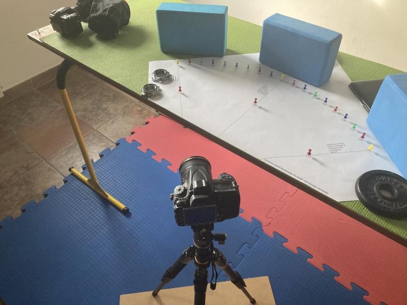 Place the camera on the tripod. Align its optical axis with the table while
looking for getting an image showing the overlapping of the three pairs of
push pins, as instructed in the print. In order to take care of the line of
pins at 90º relative to the optical axis, it may be of help to use the naked
eye to align the entrance pupil of the lens with the pins. The alignment of
the push pins only guarantees the position of the lens entrance pupil, the
leveling should be cheeked with an instrument, and the alignment between the
optical axis and the radius of the zenith push pin should be taken into
account. In practice, the latter is achieved by aligning the camera body with
the orthogonal frame made by the quarter circle.
Place the camera on the tripod. Align its optical axis with the table while
looking for getting an image showing the overlapping of the three pairs of
push pins, as instructed in the print. In order to take care of the line of
pins at 90º relative to the optical axis, it may be of help to use the naked
eye to align the entrance pupil of the lens with the pins. The alignment of
the push pins only guarantees the position of the lens entrance pupil, the
leveling should be cheeked with an instrument, and the alignment between the
optical axis and the radius of the zenith push pin should be taken into
account. In practice, the latter is achieved by aligning the camera body with
the orthogonal frame made by the quarter circle.
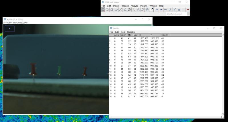
Take a photo and transfer it to the computer, open it with ImageJ, and use
the point selection tool
to digitize the push pins, starting from the zenith push pin and not skipping
any shown push pin. End with an additional point where the image meets the
surrounding black (or the last pixel in case there is not blackness because
it is not a circular hemispherical image. There is no need to follow the line
formed by the push pins). Then, use the dropdown menu Analyze>Measure to open
the window Results. To obtain the CSV, use File>Save As...
Note
To calibrate different directions, think of the fisheye image as an analog clock. To calibrate 3 o'clock, attach the camera to the tripod in landscape mode while leaving the quarter-circle at the lens's right side. To calibrate 9 o'clock, rotate the camera to put the quarter-circle at the lens's left side. To calibrate 12 and 6 o'clock, do the same but with the camera in portrait mode.
References
Díaz GM, Lang M, Kaha M (2024). “Simple calibration of fisheye lenses for hemipherical photography of the forest canopy.” Agricultural and Forest Meteorology, 352, 110020. ISSN 0168-1923, doi:10.1016/j.agrformet.2024.110020.
See Also
test_lens_coef(), crosscalibrate_lens(), extract_radiometry()
Examples
path <- system.file("external/Results_calibration.csv", package = "rcaiman")
calibration <- calibrate_lens(path)
coefficients(calibration$model)
calibration$lens_coef %>% signif(3)
calibration$horizon_radius

## Not run:
test_lens_coef(calibration$lens_coef) #MacOS and Windows tend to differ here
test_lens_coef(c(0.628, 0.0399, -0.0217))

## End(Not run)

.fp <- function(theta, lens_coef) {
  x <- lens_coef[1:5]
  x[is.na(x)] <- 0
  for (i in 1:5) assign(letters[i], x[i])
  a * theta + b * theta^2 + c * theta^3 + d * theta^4 + e * theta^5
}

plot(calibration$ds)
theta <- seq(0, pi/2, pi/180)
lines(theta, .fp(theta, coefficients(calibration$model)))
Perform chessboard segmentation
Description
Segment a raster into square regions of equal size arranged in a chessboard-like pattern.
Usage
chessboard(r, size)
Arguments
r |
numeric terra::SpatRaster. One or more layers used to drive heterogeneity. |
size |
Numeric vector of length one. Size (in pixels) of each square segment. Must be a positive integer. |
Details
This function divides the extent of a terra::SpatRaster into
non-overlapping square segments of the given size, producing a segmentation
map where each segment has a unique integer label. It can be an alternative
to sky_grid_segmentation() in special cases.
Value
terra::SpatRaster with one layer and integer values, where each unique value corresponds to a square-segment ID.
Examples
caim <- read_caim()
seg <- chessboard(caim, 20)
plot(caim$Blue)
plot(extract_feature(caim$Blue, seg))
CIE sky image
Description
Generate an image of relative radiance or luminance based on the CIE General Sky model.
Usage
cie_image(z, a, sun_angles, sky_coef)
Arguments
z |
terra::SpatRaster generated with |
a |
terra::SpatRaster generated with |
sun_angles |
named numeric vector of length two, with components
|
sky_coef |
numeric vector of length five. Parameters of the CIE sky model. |
Value
terra::SpatRaster with one layer whose pixel values
represent relative luminance or radiance across the sky hemisphere,
depending on whether the data used to obtain sky_coef was luminance
or radiance.
Note
Coefficient sets and formulation are available in cie_table.
Examples
z <- zenith_image(50, lens())
a <- azimuth_image(z)
sky_coef <- cie_table[4,1:5] %>% as.numeric()
sun_angles <- c(z = 45, a = 0)
plot(cie_image(z, a, sun_angles, sky_coef))
Set of 15 CIE Standard Skies
Description
The Commission Internationale de l’Éclairage (CIE; International Commission
on Illumination) standard (CIE 2004) defines 15
pre-calibrated sky luminance distributions, each described by a pair of
analytical functions, the gradation function
\Phi(\theta) = 1 + a \cdot \exp\left(\frac{b}{\cos\theta}\right),
and the indicatrix function
f(\chi) = 1 + c \cdot \left[ \exp(d \cdot \chi) - \exp\left(d \cdot \frac{\pi}{2}\right) \right] + e \cdot \cos^2\chi.
Combined, they can predict the relative radiance \rho_R in any sky
direction (\theta, \phi) as:
\hat{\rho_R}^{\circ}(\theta, \phi) =
\frac{\Phi(\theta) \cdot f(\chi(\theta, \phi; \theta_\odot, \phi_\odot))}
{\Phi(0) \cdot f(\chi(\theta, \phi; 0, 0))}
, where \theta is the zenith angle, \phi is the azimuth angle,
and \theta_\odot, \phi_\odot are the zenith and azimuth of the sun disk.
Usage
cie_table
Format
data.frame with 15 rows and 8 columns:
agradation function parameter.
bgradation function parameter.
cindicatrix function parameter.
dindicatrix function parameter.
eindicatrix function parameter.
indicatrix_groupfactor with six categories and numerical tags.
general_sky_typefactor with three categories:
"Overcast","Clear", and"Partly cloudy".descriptionuser-friendly description of the sky type.
Source
Li et al. (2016)
References
CIE (2004).
“ISO 15469:2004(E) / CIE S 011/E:2003 - Spatial distribution of daylight — CIE standard general sky.”
https://www.iso.org/standard/38608.html.
International Standard.
Li DHW, Lou S, Lam JC, Wu RHT (2016).
“Determining solar irradiance on inclined planes from classified CIE (International Commission on Illumination) standard skies.”
Energy, 101, 462–470.
doi:10.1016/j.energy.2016.02.054.
Calculate complementary gradients
Description
Compute three color-opponent gradients to enhance the visual separation between sky and canopy in hemispherical photographs, particularly under diffuse light or complex cloud patterns.
Usage
complementary_gradients(caim)
Arguments
caim |
numeric terra::SpatRaster with three layers named
|
Details
The method exploits chromatic differences between the red, green, and blue bands, following a simplified opponent-color logic. Each gradient is normalized by total brightness and modulated by a logistic contrast function to reduce the influence of underexposed regions:
-
"green_magenta"=(R - G + B) / (R + G + B)· logistic(brightness) -
"yellow_blue"=(-R - G + B) / (R + G + B)· logistic(brightness) -
"red_cyan"=(-R + G + B) / (R + G + B)· logistic(brightness)
The logistic(brightness) term is computed as:
\text{logistic}(x) = \frac{1}{1 + \exp\left(-\frac{x - q_{0.1}}{\mathrm{IQR}}\right)}
where q_{0.1} is the 10th percentile of brightness values
(x = R + G + B), and IQR is their interquartile range.
This weighting suppresses gradients in poorly exposed regions to reduce spurious values caused by low signal-to-noise ratios.
Value
Numeric terra::SpatRaster with three layers and the same
geometry as caim. The layers ("green_magenta", "yellow_blue",
"red_cyan") are chromatic gradients modulated by brightness.
Note
This function is part of a paper under preparation.
References
There are no references for Rd macro \insertAllCites on this help page.
Examples
## Not run:
caim <- read_caim()
com <- complementary_gradients(caim)
plot(com)

## End(Not run)
Calculate canopy openness
Description
Calculate canopy openness from a binarized hemispherical image with angular coordinates.
Usage
compute_canopy_openness(bin, z, a, m = NULL, angle_width = 10)
Arguments
bin |
logical terra::SpatRaster with one layer. A binarized
hemispherical image. See |
z |
terra::SpatRaster generated with |
a |
terra::SpatRaster generated with |
m |
logical terra::SpatRaster with one layer. A binary mask with
|
angle_width |
numeric vector of length one. Angle in deg that must
divide both 0–360 and 0–90 into an integer number of segments. Retrieve a
set of valid values by running
|
Details
Canopy openness is computed following the equation from Gonsamo et al. (2011):
CO = \sum_{i = 1}^{N} GF(\phi_i, \theta_i) \cdot \frac{\cos(\theta_{1,i}) -
 \cos(\theta_{2,i})}{n_i}
where GF(\phi_i, \theta_i) is the gap fraction in cell i,
\theta_{1,i} and \theta_{2,i} are the lower and upper zenith
angles of the cell, n_i is the number of cells in the corresponding
zenith ring, and N is the total number of cells.
When a mask is provided via the m argument, the equation is adjusted to
compensate for the reduced area of the sky vault:
CO = \frac{\sum_{i=1}^{N} GF(\phi_i, \theta_i) \cdot w_i}
{\sum_{i=1}^{N} w_i}
\quad \text{with} \quad
w_i = \frac{\cos(\theta_{1,i}) - \cos(\theta_{2,i})}{n_i}
The denominator ensures that the resulting openness value remains scale-independent. Without this normalization, masking would lead to underestimation, as the numerator alone assumes full hemispherical coverage.
Value
Numeric vector of length one, constrained to the range [0, 1].
References
Gonsamo A, Walter JN, Pellikka P (2011). “CIMES: A package of programs for determining canopy geometry and solar radiation regimes through hemispherical photographs.” Computers and Electronics in Agriculture, 79(2), 207–215. doi:10.1016/j.compag.2011.10.001.
Examples
caim <- read_caim()
z <- zenith_image(ncol(caim), lens())
a <- azimuth_image(z)
m <- select_sky_region(z, 0, 70)
bin <- binarize_with_thr(caim$Blue, thr_isodata(caim$Blue[m]))
plot(bin)
compute_canopy_openness(bin, z, a, m, 10)
Generate conventional-lens-like image
Description
Create an RGB image that resembles a photo taken with a conventional lens, using a small patch from the example hemispherical image.
Usage
conventional_lens_image()
Details
This is a fixed crop and reorientation of read_caim(). It does not perform
any re-projection. Intended for documentating functions.
The following code was used to define the region:
caim <- read_caim()
r <- caim$Blue
z <- zenith_image(ncol(caim), lens())
a <- azimuth_image(z)

m <- rast(z)
m[] <- calc_spherical_distance(
  z[] * pi / 180,
  a[] * pi / 180,
  1,# hinge-angle
  90 * pi / 180
)
m <- !binarize_with_thr(m, 30 * pi / 180)
m[is.na(z)] <- 0
m

x11()
plot(m * caim$Blue)
za <- click(c(z, a))
za
row_col <- row_col_from_zenith_azimuth(z, a, za[,1], za[,2])
plot(caim$Blue)
points(row_col$col, nrow(caim) - row_col$row, col = 2, pch = 10)
mn_y <- min(nrow(caim) -row_col$row)
mx_y <- max(nrow(caim) -row_col$row)
mn_x <- min(row_col$col)
mx_x <- max(row_col$col)
r <- terra::crop(caim$Blue, terra::ext(mn_x, mx_x, mn_y, mx_y))
plot(r)
Value
Three-layer terra::SpatRaster with bands in RGB order.
See Also
Examples
conventional_lens_image()
Correct vignetting effect
Description
Apply a vignetting correction to an image using a polynomial model.
Usage
correct_vignetting(r, z, lens_coef_v)
Arguments
r |
terra::SpatRaster of one or more layers (e.g., RGB channels or binary masks) in fisheye projection. |
z |
terra::SpatRaster generated with |
lens_coef_v |
numeric vector. Coefficients of the vignetting function
|
Details
Vignetting is the gradual reduction of image brightness toward the periphery. This function corrects it by applying a device-specific correction as a function of the zenith angle at each pixel.
Value
terra::SpatRaster with the same content as r but with
pixel values adjusted to correct for vignetting, preserving all other
properties (layers, names, extent, and CRS).
Examples
## Not run:
path <- system.file("external/APC_0836.jpg", package = "rcaiman")
caim <- read_caim(path)
z <- zenith_image(2132, lens("Olloclip"))
a <- azimuth_image(z)
zenith_colrow <- c(1063, 771)

caim <- expand_noncircular(caim, z, zenith_colrow)
m <- !is.na(caim$Red) & !is.na(z)
caim[!m] <- 0

bin <- binarize_with_thr(caim$Blue, thr_isodata(caim$Blue[m]))
display_caim(caim$Blue, bin)

caim <- invert_gamma_correction(caim, 2.2)
caim <- correct_vignetting(caim, z, c(-0.0546, -0.561, 0.22)) %>%
        normalize_minmax()

## End(Not run)
Crop a canopy image
Description
Extracts a rectangular region of interest (ROI) from a canopy image. This
function complements read_caim() and read_caim_raw().
Usage
crop_caim(r, upper_left = NULL, width = NULL, height = NULL)
Arguments
r |
|
upper_left |
numeric vector of length two. Pixel coordinates of the
upper-left corner of the ROI, in the format |
width, height |
numeric vector of length one. Size (in pixels) of the rectangular ROI to read. |
Value
terra::SpatRaster object containing the same layers and values
as r but restricted to the selected ROI, preserving all other properties.
Note
rcaiman uses terra without geographic semantics: rasters are kept with
unit resolution (cell size = 1) and a standardized extent
ext(0, ncol, 0, nrow) with CRS EPSG:7589.
Examples
caim <- read_caim()
ncell(caim)
caim <- crop_caim(caim, c(231,334), 15, 10)
ncell(caim)
Cross-calibrate lens
Description
Given two photographs taken from the same point (matching entrance pupils and
aligned optical axes), with calibrated and uncalibrated cameras, derives a
polynomial projection for the uncalibrated device. Intended for cases where a
camera calibrated with a method of higher accuracy than calibrate_lens() is
available, or when there is a main camera to which all other devices should
be adjusted.
Points must be digitized in tandem with ImageJ and saved as CSV files.
See calibrate_lens() for background and general concepts.
Usage
crosscalibrate_lens(
  path_to_csv_uncal,
  path_to_csv_cal,
  zenith_colrow_uncal,
  zenith_colrow_cal,
  diameter_cal,
  lens_coef,
  degree = 3
)
Arguments
path_to_csv_uncal, path_to_csv_cal |
character vectors of length one. Paths to CSV files created with ImageJ’s point selection tool (uncalibrated and calibrated images, respectively). |
zenith_colrow_uncal, zenith_colrow_cal |
numeric vectors of length two.
Raster coordinates of the zenith for the uncalibrated and calibrated
images; see |
diameter_cal |
numeric vector of length one. Image diameter (pixels) of the calibrated camera. |
lens_coef |
numeric vector. Lens projection coefficients of the calibrated camera. |
degree |
numeric vector of length one. Polynomial degree for the uncalibrated model fit (default 3). |
Details
Estimate a lens projection for an uncalibrated camera by referencing a calibrated camera photographed from the exact same location.
Value
List with components:
dsdata.framewith zenith angle (theta, radians) and pixel radius (px) from the uncalibrated camera.modellmobject: polynomial fit ofpx~theta.horizon_radiusnumeric vector of length one. Pixel radius at 90 deg.
lens_coefnumeric vector. Distortion coefficients normalized by
horizon_radius.
See Also
calibrate_lens(), calc_zenith_colrow()
Defuzzify a fuzzy classification
Description
Converts fuzzy membership values into a binary classification using a regional approach that preserves aggregation consistency between the fuzzy and binary representations.
Usage
defuzzify(mem, segmentation)
Arguments
mem |
numeric terra::SpatRaster of one layer. Degree of membership in a fuzzy classification. |
segmentation |
single-layer terra::SpatRaster with integer values. |
Details
The conversion is applied within segments defined by segmentation,
ensuring that, in each segment, the aggregated Boolean result matches the
aggregated fuzzy value. This approach is well suited for converting subpixel
estimates, such as gap fraction, into binary outputs.
Value
Logical terra::SpatRaster of the same dimensions as mem,
where each pixel value represents the binary version of mem after
applying the regional defuzzification procedure.
Note
This method is also available in the HSP software package. See
hsp_compat().
Examples
## Not run:
caim <- read_caim()
r <- caim$Blue
z <- zenith_image(ncol(caim), lens())
a <- azimuth_image(z)

path <- system.file("external/example.txt", package = "rcaiman")
sky_cie <- read_sky_cie(gsub(".txt", "", path), z, a)

sky_above <- ootb_sky_above(sky_cie$model$rr$sky_points, z, a, sky_cie)

ratio <- r / sky_above$dn_raster
ratio <- normalize_minmax(ratio, 0, 1, TRUE)
plot(ratio)
g <- sky_grid_segmentation(z, a, 10)
bin2 <- defuzzify(ratio, g)
plot(bin2) # unsatisfactory results due to light conditions

## End(Not run)
Display a canopy image
Description
Wrapper for EBImage::display() that streamlines the visualization of
canopy images, optionally overlaying binary masks and segmentation borders.
It is intended for quick inspection of processed or intermediate results in
a graphical viewer.
Usage
display_caim(caim = NULL, bin = NULL, g = NULL)
Arguments
caim |
terra::SpatRaster. Typically the output of |
bin |
logical terra::SpatRaster with one layer. A binarized
hemispherical image. See |
g |
single-layer terra::SpatRaster with integer values. Sky
segmentation map produced by |
Value
Invisible NULL. Called for side effects (image viewer popup).
Examples
## Not run:
caim <- read_caim()
z <- zenith_image(ncol(caim), lens())
r <- normalize_minmax(caim$Blue)
g <- ring_segmentation(z, 30)
bin <- binarize_by_region(r, g, method = "thr_isodata")
display_caim(caim$Blue, bin, g)

## End(Not run)
Estimate sun angular coordinates
Description
Estimates the sun’s zenith and azimuth angles (deg) from a canopy hemispherical photograph, using either direct detection of the solar disk or indirect cues from the circumsolar region.
Usage
estimate_sun_angles(
  r,
  z,
  a,
  bin,
  g,
  angular_radius_sun = 30,
  method = "assume_obscured"
)
Arguments
r |
numeric terra::SpatRaster of one layer. Typically the blue band of a canopy image. |
z |
terra::SpatRaster generated with |
a |
terra::SpatRaster generated with |
bin |
logical terra::SpatRaster of one layer. Binary image where
|
g |
single-layer terra::SpatRaster with integer values. Sky
segmentation map produced by |
angular_radius_sun |
numeric vector of length one. Maximum angular radius (in degrees) used to define the circumsolar region. |
method |
character vector of length one. Estimation mode:
|
Details
This function can operate under two alternative assumptions for estimating the sun position:
- Veiled sun
The solar disk is visible or partially obscured; the position is inferred from localized brightness peaks.
- Obscured sun
The solar disk is not visible; the position is inferred from radiometric and spatial cues aggregated over the circumsolar region.
When method = "assume_veiled", g and angular_radius_sun are ignored.
Estimates refer to positions above the horizon; therefore, estimated angles
may require further manipulation if the photograph was acquired under
crepuscular light.
Value
Named numeric vector of length two, with names z and a,
representing the sun’s zenith and azimuth angles (in degrees).
Note
A scientific article presenting and validating this method is currently under preparation.
Examples
## Not run:
caim <- read_caim()
z <- zenith_image(ncol(caim), lens())
a <- azimuth_image(z)
m <- !is.na(z)
r <- caim$Blue

bin <- binarize_by_region(r, ring_segmentation(z, 15), "thr_isodata") &
  select_sky_region(z, 0, 88)

g <- sky_grid_segmentation(z, a, 10)
sun_angles <- estimate_sun_angles(r, z, a, bin, g,
                                  angular_radius_sun = 30)
row_col <- row_col_from_zenith_azimuth(z, a,
                                       sun_angles["z"],
                                       sun_angles["a"])
plot(caim$Blue)
points(row_col[1,2], nrow(caim) - row_col[1,1], col = "yellow",
       pch = 8, cex = 3)

## End(Not run)
Expand non-circular
Description
Add NA margins to a hemispherical photograph to align radiance at the zenith
with the image center. In this context, “zenith” denotes the location in the image
that corresponds to the projection of the vertical direction when the optical
axis is aligned vertically. Intended for non-circular images.
Usage
expand_noncircular(caim, z, zenith_colrow)
Arguments
caim |
terra::SpatRaster. Typically the output of |
z |
terra::SpatRaster generated with |
zenith_colrow |
numeric vector of length two. Raster coordinates of the
zenith (column, row). See |
Value
terra::SpatRaster with the same layers and pixel values as caim,
but with NA margins added to center the zenith.
Note
rcaiman uses terra without geographic semantics: rasters are kept with
unit resolution (cell size = 1) and a standardized extent
ext(0, ncol, 0, nrow) with CRS EPSG:7589.
Examples
## Not run:
# Non-circular fisheye images from a smartphone with an auxiliary Lens
# (also applicable to non-circular fisheye images from DSLR cameras)
path <- system.file("external/APC_0836.jpg", package = "rcaiman")
caim <- read_caim(path)
z <- zenith_image(2132/2,  lens("Olloclip"))
a <- azimuth_image(z)
zenith_colrow <- c(1063, 771)/2
caim <- expand_noncircular(caim, z, zenith_colrow)
plot(caim$Blue, col = seq(0, 1, 1/255) %>% grey())
m <- !is.na(caim$Red) & !is.na(z)
plot(m, add = TRUE, alpha = 0.3, legend = FALSE)

## End(Not run)
Extract digital numbers from sky points
Description
Obtain digital numbers from a raster at positions defined by sky points, with optional local averaging.
Usage
extract_dn(r, sky_points, use_window = TRUE)
Arguments
r |
terra::SpatRaster. Image from which |
sky_points |
|
use_window |
logical of length one. If |
Details
Wraps terra::extract() to support a 3 \times 3 window centered on
each target pixel (local mean). When it is disabled, only the central
pixel value is retrieved.
Value
data.frame containing the original sky_points plus one column per
layer in r (named after the layers).
Note
For instructions on manually digitizing sky points, see the “Digitizing sky
points with ImageJ” and “Digitizing sky points with QGIS” sections in
fit_cie_model().
See Also
Examples
## Not run:
caim <- read_caim()
r <- caim$Blue
z <- zenith_image(ncol(caim), lens())
a <- azimuth_image(z)

# See fit_cie_model() for details on below file
path <- system.file("external/sky_points.csv",
                    package = "rcaiman")
sky_points <- read.csv(path)
sky_points <- sky_points[c("Y", "X")]
colnames(sky_points) <- c("row", "col")
head(sky_points)
plot(caim$Blue)
points(sky_points$col, nrow(caim) - sky_points$row, col = 2, pch = 10)

sky_points <- extract_dn(caim, sky_points)
head(sky_points)

# To aggregate DNs across points (excluding 'row' and 'col'):
apply(sky_points[, -(1:2)], 2, mean, na.rm = TRUE)

## End(Not run)
Extract feature
Description
Extract a numeric or logical summary from segmented raster regions using a user-defined reducer, returning one value per segment as a raster map or a named vector.
Usage
extract_feature(
  r,
  segmentation,
  fun = mean,
  return = "raster",
  ignore_label_0 = TRUE
)
Arguments
r |
numeric terra::SpatRaster with one layer. |
segmentation |
single-layer terra::SpatRaster. Segmentation map
of r, typically created with functions such as |
fun |
function taking a numeric/logical vector and returning a single
numeric or logical value (default |
return |
character of length one. Either |
ignore_label_0 |
logical of length one. If |
Details
Segments labeled 0 can be ignored via ignore_label_0 = TRUE. The
function in fun must return a single numeric or logical value for any input
vector (e.g., mean, median, or a custom reducer).
Value
If return = "raster", a terra::SpatRaster where each pixel
holds its segment’s feature value. If return = "vector", a named numeric
(or logical) vector with one value per segment.
Examples
r <- read_caim()
z <- zenith_image(ncol(r),lens())
a <- azimuth_image(z)
g <- sky_grid_segmentation(z, a, 10)
print(extract_feature(r$Blue, g, return = "vector"))
# plot(extract_feature(r$Blue, g, return = "raster"))
Extract radiometry data for calibration
Description
Buid a datasets for vignetting modeling by sistematically extracting
radiometry from images taken with the aid of a portable light source and the
calibration board detailed in calibrate_lens().
Usage
extract_radiometry(l, size_px = NULL)
Arguments
l |
list of preprocessed images (terra::SpatRaster) suitable for radiometry sampling. Images must comply with the equidistant projection. |
size_px |
numeric vector of length one. Diameter (pixels) of the
circular sampling area at the image center; off-center, the sampled region
becomes an ellipse under the equidistant projection. If |
Value
data.frame con dos columnas:
thetazenith angle en radianes.
radiometrydigital number normalizado.
Guidance
Lenses have the inconvenient property of increasingly attenuating light along the direction orthogonal to the optical axis. This phenomenon is known as the vignetting effect and varies with lens model and aperture setting. The method outlined here, known as the simple method, is explained in details in Díaz et al. (2024). Next explanation might serve mostly as a quick recap of it.
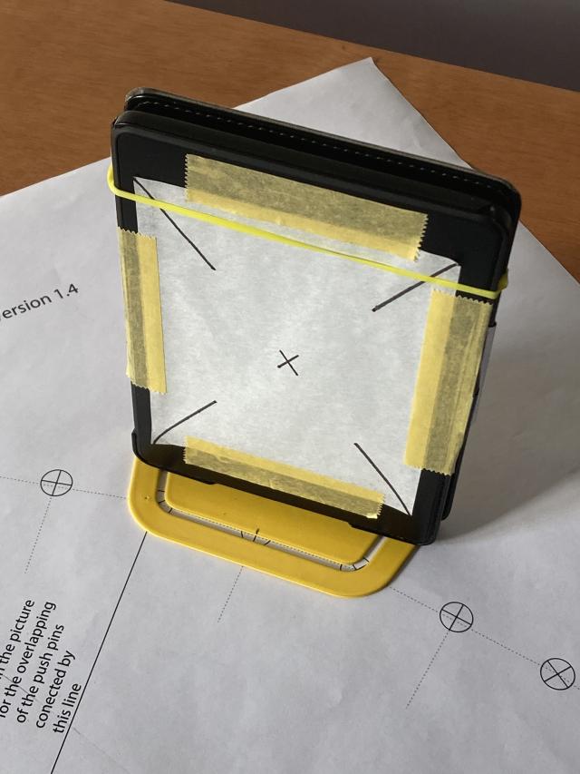
The development of the simple method was done with a Kindle Paperwhite eBooks
reader of 6" with built-in light. However, an iPhone 6 plus was also tested
in the early stages of development and no substantial differences were
observed. A metal bookends desk book holder was used to fasten the eBook
reader upright and a semi-transparent paper to favor a Lambertian light
distribution. In addition, the latter was used to draw on in order to
guide pixel sampling. The book holder also facilitated the alignment of the
screen with the dotted lines of the printed quarter-circle.
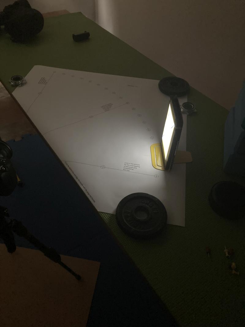
 As a general guideline, a wide variety of mobile devices could be used as
light sources, but if scattered data points are obtained with it, then other
light sources should be tested in order to double check that the light
quality is not the reason for points scattering.
As a general guideline, a wide variety of mobile devices could be used as
light sources, but if scattered data points are obtained with it, then other
light sources should be tested in order to double check that the light
quality is not the reason for points scattering.
With the room only illuminated by the portable light source, nine photographs
should be taken with the light source located in the equivalent to 0, 10, 20,
30, 40, 50, 60, 70, and 80 degrees of zenith angle, respectively. Camera
configuration should be in manual mode and set with the aperture (f/number)
for which a vignetting function is required. The shutter speed should be
regulated to obtain light-source pixels with middle grey values. The nine
photographs should be taken without changing the camera configuration and
the light conditions.
 This code exemplifies how to use the function to obtain data and base R
functions to obtain the vignetting function (
This code exemplifies how to use the function to obtain data and base R
functions to obtain the vignetting function (f_v).
zenith_colrow <- c(1500, 997)
diameter <- 947*2
z <- zenith_image(diameter, c(0.689, 0.0131, -0.0295))
a <- azimuth_image(z)

.read_raw <- function(path_to_raw_file) {
  r <- read_caim_raw(path_to_raw_file, only_blue = TRUE)
  r <- crop_caim(r, zenith_colrow - diameter/2, diameter, diameter)
  r <- fisheye_to_equidistant(r, z, a, m, radius = diameter/2,
                              k = 1, p = 1, rmax = 100)
}

l <- Map(.read_raw, dir("raw/up/", full.names = TRUE))
up_data <- extract_radiometry(l)
l <- Map(.read_raw, dir("raw/down/", full.names = TRUE))
down_data <- extract_radiometry(l)
l <- Map(.read_raw, dir("raw/right/", full.names = TRUE))
right_data <- extract_radiometry(l)
l <- Map(.read_raw, dir("raw/left/", full.names = TRUE))
left_data <- extract_radiometry(l)

ds <- rbind(up_data, down_data, right_data, left_data)

plot(ds, xlim = c(0, pi/2), ylim= c(0.5,1.05),
      col = c(rep(1,9),rep(2,9),rep(3,9),rep(4,9)))
legend("bottomleft", legend = c("up", "down", "right", "left"),
       col = 1:4, pch = 1)

fit <- lm((1 - ds$radiometry) ~ poly(ds$theta, 3, raw = TRUE) - 1)
summary(fit)
coef <- -fit$coefficients #did you notice the minus sign?
.fv <- function(x) 1 + coef[1] * x + coef[2] * x^2 + coef[3] * x^3
curve(.fv, add = TRUE, col = 2)
coef
Once one of the aperture settings is calibrated, it can be used to calibrate all the rest. To do so, the equipment should be used to take photographs in all desired exposition and without moving the camera, including the aperture already calibrated and preferably under an open sky in stable diffuse light conditions. Below code can be used as a template.
zenith_colrow <- c(1500, 997)
diameter <- 947*2
z <- zenith_image(diameter, c(0.689, 0.0131, -0.0295))
a <- azimuth_image(z)

files <- dir("raw/", full.names = TRUE)
l <- list()
for (i in seq_along(files)) {
  if (i == 1) {
    # because the first aperture was the one already calibrated
    .read_raw <- function(path_to_raw_file) {
        r <- read_caim_raw(path_to_raw_file, only_blue = TRUE)
        r <- crop_caim(r, zenith_colrow - diameter/2, diameter, diameter)
        r <- correct_vignetting(r, z, c(0.0302, -0.320, 0.0908))
        r <- fisheye_to_equidistant(r, z, a, m, radius = diameter/2,
                                    k = 1, p = 1, rmax = 100)
      }
  } else {
      .read_raw <- function(path_to_raw_file) {
          r <- read_caim_raw(path_to_raw_file, only_blue = TRUE)
          r <- crop_caim(r, zenith_colrow - diameter/2, diameter, diameter)
          r <- fisheye_to_equidistant(r, z, a, m, radius = diameter/2,
                                      k = 1, p = 1, rmax = 100)
        }
  }
  l[[i]] <- .read_raw(files[i])
}

ref <- l[[1]]
rings <- ring_segmentation(zenith_image(ncol(ref), lens()), 3)
theta <- seq(1.5, 90 - 1.5, 3) * pi/180

.fun <- function(r) {
  r <- extract_feature(r, rings, return = "vector")
  r/r[1]
}

l <- Map(.fun, l)

.fun <- function(x) {
  x / l[[1]][] # because the first is the one already calibrated
}
radiometry <- Map(.fun, l)

l <- list()
for (i in 2:length(radiometry)) {
  l[[i-1]] <- data.frame(theta = theta, radiometry = radiometry[[i]][])
}
ds <- l[[1]]
head(ds)
The result is one dataset (ds) for each file. This is all what it is needed before using base R functions to fit a vignetting function
Note
This function does not fit the vignetting function itself. The output is a dataset to be used in subsequent modeling steps. See above sections for guidance.
References
Díaz GM, Lang M, Kaha M (2024). “Simple calibration of fisheye lenses for hemipherical photography of the forest canopy.” Agricultural and Forest Meteorology, 352, 110020. ISSN 0168-1923, doi:10.1016/j.agrformet.2024.110020.
Extract digital numbers at sky points and normalize by estimated zenith radiance
Description
Compute relative radiance at selected sky points by dividing their digital numbers (DN) by an estimated zenith DN.
Usage
extract_rr(r, z, a, sky_points, no_of_points = 3, use_window = TRUE)
Arguments
r |
terra::SpatRaster. Raster supplying the DN values; must
share rows and columns with the image used to obtain |
z |
terra::SpatRaster generated with |
a |
terra::SpatRaster generated with |
sky_points |
|
no_of_points |
numeric vector of length one or |
use_window |
logical of length one. If |
Value
List with named elements:
zenith_dnnumeric. Estimated DN at the zenith.
sky_pointsdata.framewith columnsrow,col,a,z,dn, andrr(pixel location, angular coordinates, extracted DN, and relative radiance). Ifno_of_pointsisNULL,zenith_dn = 1anddn = rr.
Examples
## Not run:
caim <- read_caim()
z <- zenith_image(ncol(caim), lens())
a <- azimuth_image(z)

# See fit_cie_model() for details on the CSV file
path <- system.file("external/sky_points.csv",
                    package = "rcaiman")
sky_points <- read.csv(path)
sky_points <- sky_points[c("Y", "X")]
colnames(sky_points) <- c("row", "col")
head(sky_points)

plot(caim$Blue)
points(sky_points$col, nrow(caim) - sky_points$row, col = 2, pch = 10)
rr <- extract_rr(caim$Blue, z, a, sky_points, 1)
points(rr$sky_points$col, nrow(caim) - rr$sky_points$row, col = 3, pch = 0)

## End(Not run)
Extract sky points
Description
Sample representative sky pixels for use in model fitting or interpolation.
Usage
extract_sky_points(r, bin, g, dist_to_black = 3, method = "grid")
Arguments
r |
numeric terra::SpatRaster of one layer. Typically the blue band of a canopy image. |
bin |
logical terra::SpatRaster of one layer. Binary image where
|
g |
numeric terra::SpatRaster of one layer. Segmentation grid,
usually built with |
dist_to_black |
numeric vector of length one or |
method |
character vector of length one. Sampling method; either
|
Details
Two sampling strategies are provided:
"grid"select one sky point per cell of a segmentation grid (
g) as the brightest pixel markedTRUEinbin, provided the cell’s white pixel count exceeds one fourth of the mean across valid cells."local_max"detect local maxima within a fixed
9 \times 9window, restricted to pixels markedTRUEinbin, after removing patches of connectedTRUEpixels that are implausible based on fixed area/size thresholds. Each detected maximum is taken as a sky point.
Use "grid" to promote an even, representative spatial distribution (good
for model fitting), and "local_max" to be exhaustive for interpolation.
Value
data.frame with columns row and col.
Examples
## Not run:
caim <- read_caim()
z <- zenith_image(ncol(caim), lens())
a <- azimuth_image(z)
m <- !is.na(z)
r <- caim$Blue

bin <- binarize_by_region(r, ring_segmentation(z, 15), "thr_isodata") &
  select_sky_region(z, 0, 88)

g <- sky_grid_segmentation(z, a, 10)
sky_points <- extract_sky_points(r, bin, g,
                                 dist_to_black = 3)
plot(bin)
points(sky_points$col, nrow(caim) - sky_points$row, col = 2, pch = 10)

## End(Not run)
Fisheye to equidistant
Description
Reproject a hemispherical image from fisheye to equidistant projection (also known as polar projection) to standardize its geometry for subsequent analysis and comparison between images.
Usage
fisheye_to_equidistant(r, z, a, m, radius = NULL, k = 1, p = 1, rmax = 100)
Arguments
r |
terra::SpatRaster of one or more layers (e.g., RGB channels or binary masks) in fisheye projection. |
z |
terra::SpatRaster generated with |
a |
terra::SpatRaster generated with |
m |
logical terra::SpatRaster with one layer. A binary mask with
|
radius |
numeric vector of length one. Radius (in pixels) of the
reprojected hemispherical image. Must be an integer value (no decimal
part). If |
k, p, rmax |
numeric vector of length one. Parameters passed to
|
Details
Pixel values and coordinates are treated as 3D points and reprojected
using Cartesian interpolation. Internally, this function uses
lidR::knnidw() as interpolation engine, so arguments k, p, and
rmax are passed to it without modification.
Value
terra::SpatRaster with the same number of layers as r,
reprojected to equidistant projection with circular shape and radius
given by 'radius
Examples
## Not run:
path <- system.file("external/APC_0836.jpg", package = "rcaiman")
caim <- read_caim(path)
calc_diameter(c(0.801, 0.178, -0.179), 1052, 86.2)
z <- zenith_image(2216,  c(0.801, 0.178, -0.179))
a <- azimuth_image(z)
zenith_colrow <- c(1063, 771)

caim <- expand_noncircular(caim, z, zenith_colrow)
m <- !is.na(caim$Red) & select_sky_region(z, 0, 86.2)
caim[!m] <- 0
m2 <- fisheye_to_equidistant(m, z, a, !is.na(z), radius = 600)
m2 <- binarize_with_thr(m2, 0.5) #to turn it logical
caim2[!m2] <- 0

plot(caim)

## End(Not run)
Fisheye to panoramic
Description
Reprojects a fisheye (hemispherical) image into a panoramic view using a cylindrical projection. The output is standardized so that rows correspond to zenith angle bands and columns to azimuthal sectors.
Usage
fisheye_to_pano(r, z, a, fun = mean, angle_width = 1)
Arguments
r |
terra::SpatRaster of one or more layers (e.g., RGB channels or binary masks) in fisheye projection. |
z |
terra::SpatRaster generated with |
a |
terra::SpatRaster generated with |
fun |
function taking a numeric/logical vector and returning a single
numeric or logical value (default |
angle_width |
numeric vector of length one. Angle in deg that must
divide both 0–360 and 0–90 into an integer number of segments. Retrieve a
set of valid values by running
|
Details
This function computes a cylindrical projection by aggregating pixel values
according to their zenith and azimuth angles. Internally, it creates a
segmentation grid with sky_grid_segmentation() and applies
extract_feature() to compute a summary statistic (e.g., mean) of pixel
values within each cell.
Value
terra::SpatRaster with rows representing zenith angle bands and
columns representing azimuthal sectors. The number of layers and names
matches that of the input r.
Note
An early version of this function was used in Díaz et al. (2021).
References
Díaz GM, Negri PA, Lencinas JD (2021). “Toward making canopy hemispherical photography independent of illumination conditions: A deep-learning-based approach.” Agricultural and Forest Meteorology, 296, 108234. doi:10.1016/j.agrformet.2020.108234.
Examples
## Not run:
caim <- read_caim()
z <- zenith_image(ncol(caim), lens())
a <- azimuth_image(z)
pano <- fisheye_to_pano(caim, z, a)
plotRGB(pano %>% normalize_minmax() %>% multiply_by(255))

## End(Not run)
Fit CIE sky model
Description
Fit the CIE sky model to data sampled from a canopy photograph using general-purpose optimization.
Usage
fit_cie_model(
  rr,
  sun_angles,
  custom_sky_coef = NULL,
  std_sky_no = NULL,
  general_sky_type = NULL,
  method = c("Nelder-Mead", "BFGS", "CG", "SANN")
)
Arguments
rr |
list, typically the output of
|
sun_angles |
named numeric vector of length two, with components
|
custom_sky_coef |
numeric vector of length five, or numeric matrix with five columns. Custom starting coefficients for optimization. If not provided, coefficients are initialized from standard skies. |
std_sky_no |
numeric vector. Standard sky numbers as in cie_table. If not provided, all are used. |
general_sky_type |
character vector of length one. Must be |
method |
character vector. Optimization methods passed to
|
Details
The method is based on Lang et al. (2010).
For best results, the input data should show a linear relation between
digital numbers and the amount of light reaching the sensor. See
extract_radiometry() and read_caim_raw() for details.
As a compromise solution, invert_gamma_correction() can be used.
Value
List with the following components:
rrThe input
rrwith an addedpredcolumn insky_points, containing predicted values.opt_resultList returned by
stats::optim().coefNumeric vector of length five. CIE model coefficients.
sun_anglesNumeric vector of length two. Sun zenith and azimuth (degrees).
methodCharacter string. Optimization method used.
startNumeric vector of length five. Starting parameters.
metricNumeric value. Mean squared deviation as in Gauch et al. (2003).
Background
This function is based on Lang et al. (2010). In theory,
the best result would be obtained with data showing a linear relation between
digital numbers and the amount of light reaching the sensor. See
extract_radiometry() and read_caim_raw() for further details. As a
compromise solution, invert_gamma_correction() can be used.
Digitizing sky points with ImageJ
The point selection tool of ‘ImageJ’ software can be used to manually digitize points and create a CSV file from which to read coordinates (see Examples). After digitizing the points on the image, this is a recommended workflow: 1. Use the dropdown menu Analyze > Measure to open the Results window. 2. Use File > Save As... to obtain the CSV file.
Use this code to create the input sky_points from ImageJ data:
sky_points <- read.csv(path)
sky_points <- sky_points[c("Y", "X")]
colnames(sky_points) <- c("row", "col")
Digitizing sky points with QGIS
To use the QGIS software to manually digitize points, drag and drop the image in an empty project, create an new vector layer, digitize points manually, save the editions, and close the project.
To create the new vector layer, this is a recommended workflow:
Fo to the dropdown menu Layer > Create Layer > New Geopackage Layer...
Choose "point" in the Geometry type dropdown list
Make sure the CRS is EPSG:7589.
Click on the Toogle Editing icon
Click on the Add Points Feature icon.
Use this code to create the input sky_points from QGIS data:
sky_points <- terra::vect(path)
sky_points <- terra::extract(caim, sky_points, cells = TRUE)
sky_points <- terra::rowColFromCell(caim, sky_points$cell) %>% as.data.frame()
colnames(sky_points) <- c("row", "col")
References
Gauch HG, Hwang JTG, Fick GW (2003).
“Model evaluation by comparison of model‐based predictions and measured values.”
Agronomy Journal, 95(6), 1442–1446.
ISSN 1435-0645, doi:10.2134/agronj2003.1442.
Lang M, Kuusk A, Mõttus M, Rautiainen M, Nilson T (2010).
“Canopy gap fraction estimation from digital hemispherical images using sky radiance models and a linear conversion method.”
Agricultural and Forest Meteorology, 150(1), 20–29.
doi:10.1016/j.agrformet.2009.08.001.
Examples
## Not run:
caim <- read_caim()
z <- zenith_image(ncol(caim), lens())
a <- azimuth_image(z)

# Manual method following Lang et al. (2010)
path <- system.file("external/sky_points.csv",
                    package = "rcaiman")
sky_points <- read.csv(path)
sky_points <- sky_points[c("Y", "X")]
colnames(sky_points) <- c("row", "col")
head(sky_points)
plot(caim$Blue)
points(sky_points$col, nrow(caim) - sky_points$row, col = 2, pch = 10)

# x11()
# plot(caim$Blue)
# sun_angles <- click(c(z, a), 1) %>% as.numeric()
sun_angles <- c(z = 49.5, a = 27.4) #taken with above lines then hardcoded

sun_row_col <- row_col_from_zenith_azimuth(z, a,
                                           sun_angles["z"],
                                           sun_angles["a"])
points(sun_row_col[2], nrow(caim) - sun_row_col[1],
       col = "yellow", pch = 8, cex = 3)

rr <- extract_rr(caim$Blue, z, a, sky_points)

set.seed(7)
model <- fit_cie_model(rr, sun_angles,
                           general_sky_type = "Clear")

plot(model$rr$sky_points$rr, model$rr$sky_points$pred)
abline(0,1)
lm(model$rr$sky_points$pred~model$rr$sky_points$rr) %>% summary()

sky <- cie_image(z, a, model$sun_angles, model$coef) * model$rr$zenith_dn

plot(sky)
ratio <- caim$Blue/sky
plot(ratio)
plot(ratio > 1.05)
plot(ratio > 1.15)

## End(Not run)
Fit cone-shaped model
Description
Fit a polynomial model to predict relative radiance from spherical coordinates using data sampled from a canopy photograph.
Usage
fit_coneshaped_model(sky_points, method = "zenith_n_azimuth")
Arguments
sky_points |
|
method |
character. Model type to fit:
|
Details
This model requires only sky_points, making it useful in workflows where
sun position cannot be reliably estimated, such as in apply_by_direction().
Otherwise, fit_cie_model() is a better choice.
Depending on method, it can fit:
- A zenith-only quadratic model
sDN = a + b\theta + c\theta^2- A zenith-plus-azimuth model, adding sinusoidal terms
sDN = a + b\theta + c\theta^2 + d\sin(\phi) + e\cos(\phi)
See Díaz and Lencinas (2018) for details on the full model.
Value
List with the following components:
funFunction taking
zenithandazimuth(degrees) and returning predicted relative radiance.modellmobject fitted bystats::lm().
Returns NULL (with a warning) if the number of input points is fewer than 20.
References
Díaz GM, Lencinas JD (2018). “Model-based local thresholding for canopy hemispherical photography.” Canadian Journal of Forest Research, 48(10), 1204–1216. doi:10.1139/cjfr-2018-0006.
Examples
## Not run:
caim <- read_caim()
z <- zenith_image(ncol(caim), lens())
a <- azimuth_image(z)
m <- !is.na(z)
r <- caim$Blue

bin <- binarize_by_region(r, ring_segmentation(z, 15), "thr_isodata") &
  select_sky_region(z, 0, 88)

g <- sky_grid_segmentation(z, a, 10, first_ring_different = TRUE)
sky_points <- extract_sky_points(r, bin, g, dist_to_black = 3)
plot(bin)
points(sky_points$col, nrow(caim) - sky_points$row, col = 2, pch = 10)
rr <- extract_rr(r, z, a, sky_points)

model <- fit_coneshaped_model(rr$sky_points)
summary(model$model)
sky_cs <- model$fun(z, a) * rr$zenith_dn
plot(sky_cs)

z_mini <- zenith_image(50, lens())
sky_cs <- model$fun(z_mini, azimuth_image(z_mini))
persp(sky_cs, theta = 90, phi = 20)


## End(Not run)
Fit a trend surface to sky digital numbers
Description
Fits a trend surface to sky digital numbers using spatial::surf.ls() as
the computational workhorse.
Usage
fit_trend_surface(sky_points, r, np = 6, col_id = "dn", extrapolate = FALSE)
Arguments
sky_points |
|
r |
numeric terra::SpatRaster with one layer. Image from which
|
np |
degree of polynomial surface |
col_id |
numeric or character vector of length one. The name or position
of the column in |
extrapolate |
logical vector of length one. If |
Details
This function models the variation in digital numbers across the sky dome
by fitting a polynomial surface in Cartesian space. It is intended to
capture smooth large-scale gradients and is more effective when called
via apply_by_direction().
Value
List with named elements:
rasterterra::SpatRaster containing the fitted surface.
modelobject of class
trlsreturned byspatial::surf.ls().r2numeric value giving the coefficient of determination (R
^2) of the fit.
References
There are no references for Rd macro \insertAllCites on this help page.
Examples
## Not run:
caim <- read_caim()
z <- zenith_image(ncol(caim), lens())
a <- azimuth_image(z)
m <- !is.na(z)
r <- caim$Blue

bin <- binarize_by_region(r, ring_segmentation(z, 15), "thr_isodata") &
  select_sky_region(z, 0, 88)

g <- sky_grid_segmentation(z, a, 10, first_ring_different = TRUE)
sky_points <- extract_sky_points(r, bin, g, dist_to_black = 3)
plot(bin)
points(sky_points$col, nrow(caim) - sky_points$row, col = 2, pch = 10)
sky_points <- extract_dn(r, sky_points, use_window = TRUE)

sky_s <- fit_trend_surface(sky_points, r, np = 4, col_id = 3,
                           extrapolate = TRUE)
plot(sky_s$raster)
binarize_with_thr(r/sky_s$raster, 0.5) %>% plot()

sky_s <- fit_trend_surface(sky_points, r, np = 6, col_id = 3,
                           extrapolate = FALSE)
plot(sky_s$raster)
binarize_with_thr(r/sky_s$raster, 0.5) %>% plot()

## End(Not run)
Grow black regions in a binary mask
Description
Grow black pixels in a binary mask using a kernel of user-defined size. Useful to reduce errors associated with inter-class borders.
Usage
grow_black(bin, dist_to_black)
Arguments
bin |
logical terra::SpatRaster with one layer. A binarized
hemispherical image. See |
dist_to_black |
numeric vector of length one. Buffer distance (pixels) used to expand black regions. |
Details
Expands the regions with value FALSE (typically rendered as black) in a
binary image by applying a square-shaped buffer. Any white pixels (value
TRUE) within a distance equal to or less than dist_to_black from a black
pixel will be turned black.
Value
Logical terra::SpatRaster with the same dimensions as bin. Compared
to the input bin, black regions (FALSE) have been expanded by the
specified buffer distance.
Examples
## Not run:
r <- read_caim()
bin <- binarize_with_thr(r$Blue, thr_isodata(r$Blue[]))
plot(bin)
bin <- grow_black(bin, 11)
plot(bin)

## End(Not run)
HSP compatibility functions
Description
Read and write legacy files from HSP (HemiSPherical Project Manager) projects
to interoperate with existing workflows. Intended for legacy support; not
required when working fully within rcaiman.
Usage
hsp_read_manual_input(path_to_HSP_project, img_name)

hsp_read_opt_sky_coef(path_to_HSP_project, img_name)

hsp_write_sky_points(sky_points, path_to_HSP_project, img_name)

hsp_write_sun_coord(sun_row_col, path_to_HSP_project, img_name)
Arguments
path_to_HSP_project |
character vector of length one. Path to the HSP
project folder (e.g., |
img_name |
character vector of length one (e.g., |
sky_points |
|
sun_row_col |
numeric vector of length two. Raster coordinates (row, column) of the solar disk. |
Value
See Functions
About HSP software
HSP (introduced in (Lang et al. 2013), based on the method in
(Lang et al. 2010)) runs exclusively on Windows. HSP stores
pre-processed images as PGM files in the manipulate subfolder of each
project (itself inside the projects folder).
Functions
hsp_read_manual_input()read sky marks and sun position defined manually within an HSP project; returns a named list with components
weight,max_points,angle,point_radius,sun_row_col,sky_points, andzenith_dn.hsp_read_opt_sky_coef()read optimized CIE sky coefficients from an HSP project; returns a numeric vector of length five.
hsp_write_sky_points()write a file with sky point coordinates compatible with HSP; creates a file on disk.
hsp_write_sun_coord()write a file with solar disk coordinates compatible with HSP; creates a file on disk.
References
Lang M, Kodar A, Arumäe T (2013).
“Restoration of above canopy reference hemispherical image from below canopy measurements for plant area index estimation in forests.”
Forestry Studies, 59(1), 13–27.
doi:10.2478/fsmu-2013-0008.
Lang M, Kuusk A, Mõttus M, Rautiainen M, Nilson T (2010).
“Canopy gap fraction estimation from digital hemispherical images using sky radiance models and a linear conversion method.”
Agricultural and Forest Meteorology, 150(1), 20–29.
doi:10.1016/j.agrformet.2009.08.001.
Examples
## Not run:
# NOTE: assumes the working directory is the HSP project folder (e.g., an RStudio project).

# From HSP to R in order to compare ---------------------------------------
r <- read_caim("manipulate/IMG_1013.pgm")
z <- zenith_image(ncol(r), lens())
a <- azimuth_image(z)
manual_input <- read_manual_input(".", "IMG_1013")
sun_row_col <- manual_input$sun_row_col
sun_angles <- zenith_azimuth_from_row_col(
  z, a,
  sun_row_col[1],
  sun_row_col[2]
)
sun_angles <- as.vector(sun_angles)

sky_points <- manual_input$sky_points
rr <- extract_rr(r, z, a, sky_points)
model <- fit_cie_model(rr, sun_angles)
sky <- cie_image(
  z, a,
  model$sun_angles,
  model$coef
) * model$rr$zenith_dn
plot(r / sky)

r <- read_caim("manipulate/IMG_1013.pgm")
sky_coef <- read_opt_sky_coef(".", "IMG_1013")
sky_m <- cie_image(z, a, sun_angles, sky_coef)
sky_m <- cie_sky_manual * manual_input$zenith_dn
plot(r / sky_m)

# From R to HSP  ----------------------------------------------------------
r <- read_caim("manipulate/IMG_1014.pgm")
z <- zenith_image(ncol(r), lens())
a <- azimuth_image(z)
m <- !is.na(z)
g <- sky_grid_segmentation(z, a, 10)
bin <- binarize_with_thr(caim$Blue, thr_isodata(caim$Blue[m]))
bin <- select_sky_region(z, 0, 85) & bin

sun_angles <- estimate_sun_angles(r, z, a, bin, g)
sun_row_col <- row_col_from_zenith_azimuth(
  z, a,
  sun_angles["z"],
  sun_angles["a"]
) %>% as.numeric()
write_sun_coord(sun_row_col, ".", "IMG_1014")

sky_points <- extract_sky_points(r, bin, g)
write_sky_points(sky_points, ".", "IMG_1014")

## End(Not run)
Interpolate in planar space
Description
Interpolate values from canopy photographs using inverse distance weighting (IDW) with k-nearest neighbors in image (planar) coordinates. A radius limits neighbor search.
Usage
interpolate_planar(sky_points, r, k = 3, p = 2, rmax = 200, col_id = "dn")
Arguments
sky_points |
|
r |
numeric terra::SpatRaster with one layer. Image from which
|
k, p, rmax |
numeric vector of length one. Parameters passed to
|
col_id |
numeric or character vector of length one. The name or position
of the column in |
Details
Delegates interpolation to lidR::knnidw(), passing k, p, and rmax
unchanged. Defaults follow Lang et al. (2013).
Note that rmax is given in pixels but intended to approximate 15–20 deg in
angular terms. Therefore, this value needs fine-tuning based on image
resolution and lens projection. For best results, the interpolated quantity
should be linearly related to scene radiance; see extract_radiometry() and
read_caim_raw(). For JPEG images, consider invert_gamma_correction() to reverse gamma
encoding.
Value
Numeric terra::SpatRaster with one layer and the same geometry
as r.
Note
No consistency checks are performed to ensure that sky_points and r
are geometrically compatible. Incorrect combinations may lead to invalid
outputs.
References
Lang M, Kodar A, Arumäe T (2013). “Restoration of above canopy reference hemispherical image from below canopy measurements for plant area index estimation in forests.” Forestry Studies, 59(1), 13–27. doi:10.2478/fsmu-2013-0008.
Examples
## Not run:
caim <- read_caim()
z <- zenith_image(ncol(caim), lens())
a <- azimuth_image(z)
m <- !is.na(z)
r <- caim$Blue

bin <- binarize_by_region(r, ring_segmentation(z, 15), "thr_isodata") &
  select_sky_region(z, 0, 88)

g <- sky_grid_segmentation(z, a, 10)
sky_points <- extract_sky_points(r, bin, g, dist_to_black = 3)
plot(bin)
points(sky_points$col, nrow(caim) - sky_points$row, col = 2, pch = 10)
sky_points <- extract_dn(r, sky_points)

sky <- interpolate_planar(sky_points, r, col_id = 3)
plot(sky)
plot(r/sky)

## End(Not run)
Interpolate in spherical space
Description
Interpolate values from canopy photographs using inverse distance weighting (IDW) with k-nearest neighbors, computing distances in spherical coordinates that map the sky vault. Optionally blend with a model surface to fill voids.
Usage
interpolate_spherical(
  sky_points,
  z,
  a,
  filling_source = NULL,
  w = 1,
  k = 3,
  p = 2,
  angular_radius = 20,
  rule = "any",
  size = 50
)
Arguments
sky_points |
|
z |
terra::SpatRaster generated with |
a |
terra::SpatRaster generated with |
filling_source |
optional numeric terra::SpatRaster with one
layer. Surface used to complement |
w |
numeric vector of length one. Weight assigned to |
k |
numeric vector of length one. Number of neighbors. |
p |
numeric vector of length one. Inverse distance weighting exponent. |
angular_radius |
numeric vector of length one. The maximum radius for searching k-nearest neighbors (KNN) in degrees. |
rule |
character vector of length one. Either |
size |
numeric vector of length one. Number of rows and columns of the low-resolution grid used before resampling to full resolution. |
Details
Distances are great-circle distances on the sky vault. When filling_source is
provided, local IDW estimates are blended with that surface following Eq. 6
in Lang et al. (2010). For efficiency, interpolation runs
on a temporary low-resolution grid of size size.
Value
Numeric terra::SpatRaster with one layer of interpolated
values and the geometry of z.
Note
This function assumes that sky_points and the
terra::SpatRaster inputs are spatially aligned and share the same
geometry. No checks are performed to enforce this.
References
Lang M, Kuusk A, Mõttus M, Rautiainen M, Nilson T (2010). “Canopy gap fraction estimation from digital hemispherical images using sky radiance models and a linear conversion method.” Agricultural and Forest Meteorology, 150(1), 20–29. doi:10.1016/j.agrformet.2009.08.001.
Examples
## Not run:
caim <- read_caim()
z <- zenith_image(ncol(caim), lens())
a <- azimuth_image(z)

# Manual method following Lang et al. (2010)
path <- system.file("external/sky_points.csv",
                    package = "rcaiman")
sky_points <- read.csv(path)
sky_points <- sky_points[c("Y", "X")]
colnames(sky_points) <- c("row", "col")
head(sky_points)
plot(caim$Blue)
points(sky_points$col, nrow(caim) - sky_points$row, col = 2, pch = 10)

# x11()
# plot(caim$Blue)
# sun_angles <- click(c(z, a), 1) %>% as.numeric()
sun_angles <- c(z = 49.5, a = 27.4) #taken with above lines then hardcoded

sun_row_col <- row_col_from_zenith_azimuth(z, a,
                                           sun_angles["z"],
                                           sun_angles["a"])
points(sun_row_col[2], nrow(caim) - sun_row_col[1],
       col = "yellow", pch = 8, cex = 3)

rr <- extract_rr(caim$Blue, z, a, sky_points)

set.seed(7)
model <- fit_cie_model(rr, sun_angles,
                       general_sky_type = "Clear")

sky_cie <- cie_image(z, a, model$sun_angles, model$coef)

sky_rr <- interpolate_spherical(rr$sky_points, z, a,
                                filling_source = sky_cie,
                                w = 1,
                                k = 10,
                                p = 2,
                                angular_radius = 20,
                                rule = "any",
                                size = 50)
plot(r/sky_rr/rr$zenith_dn)

## End(Not run)
Gamma back correction of JPEG images
Description
Approximates the inversion of the gamma encoding applied to JPEG images.
Usage
invert_gamma_correction(dn, gamma = 2.2)
Arguments
dn |
numeric vector or terra::SpatRaster. Digital numbers from a JPEG file (range 0–255, as per standard 8-bit encoding). |
gamma |
numeric vector of length one. Exponent applied in the inverse gamma correction (typically 2.2 for sRGB). |
Details
Digital cameras typically encode images using the sRGB color space, which applies a non-linear transformation—commonly referred to as gamma correction—to the sensor's linear luminance response. This function applies a power transformation to approximate the inverse of that encoding, restoring a response closer to linear.
Value
Same properties as dn, with values adjusted by
inverse gamma correction and rescaled to the range [0, 1].
References
There are no references for Rd macro \insertAllCites on this help page.
Examples
## Not run:
path <- system.file("external/APC_0836.jpg", package = "rcaiman")
caim <- read_caim(path)
z <- zenith_image(2132,  lens("Olloclip"))
a <- azimuth_image(z)
zenith_colrow <- c(1063, 771)

caim <- expand_noncircular(caim, z, zenith_colrow)
m <- !is.na(caim$Red) & !is.na(z)
caim[!m] <- 0

bin <- binarize_with_thr(caim$Blue, thr_isodata(caim$Blue[m]))

display_caim(caim$Blue, bin)

caim <- invert_gamma_correction(caim, 2.2)

## End(Not run)
Access the lens database
Description
Retrieve projection coefficients and field-of-view (FOV, deg) for known lenses. Coefficients expect zenith angle in radians and return relative radius.
Usage
lens(type = "equidistant", return = "coef")
Arguments
type |
Character vector of length one. Lens identifier. See Details. |
return |
Character vector of length one. Either |
Details
In upward-looking leveled hemispherical photography, the zenith corresponds to the center of a circular image whose perimeter represents the horizon, assuming a lens with a 180° field of view. The relative radius is the radial distance to a given point, expressed as a fraction of the maximum radius (i.e., the horizon). The equidistant projection model, also called polar projection, is the standard reference model, characterized by a linear relationship between zenith angle and relative radius.
Real lenses deviate from ideal projections. Following Hemisfer software, this package models deviations with polynomial functions. All angular values are in radians.
Currently available lenses:
- "equidistant"
Ideal equidistant projection (Schneider et al. 2009).
- "Nikkor_10.5mm"
AF DX Fisheye Nikkor 10.5mm f/2.8G ED (Pekin and Macfarlane 2009).
- "Nikon_FCE9"
Nikon FC-E9 converter (Díaz et al. 2024).
- "Olloclip"
Auxiliary lens for mobile devices manufactured by Olloclip (Díaz et al. 2024).
- "Nikkor_8mm"
AF–S Fisheye Nikkor 8–15mm f/3.5–4.5E ED (Díaz et al. 2024).
See calibrate_lens() for fitting new projection functions.
Value
Numeric vector. Depends on return:
- "coef"
Polynomial coefficients of the projection function (relative radius as a function of
theta, radians).- "fov"
numeric vector of length one. Maximum field of view (deg).
References
Díaz GM, Lang M, Kaha M (2024).
“Simple calibration of fisheye lenses for hemipherical photography of the forest canopy.”
Agricultural and Forest Meteorology, 352, 110020.
ISSN 0168-1923, doi:10.1016/j.agrformet.2024.110020.
Pekin B, Macfarlane C (2009).
“Measurement of crown cover and leaf area index using digital cover photography and its application to remote sensing.”
Remote Sensing, 1(4), 1298–1320.
doi:10.3390/rs1041298.
Schneider D, Schwalbe E, Maas H (2009).
“Validation of geometric models for fisheye lenses.”
ISPRS Journal of Photogrammetry and Remote Sensing, 64(3), 259–266.
doi:10.1016/j.isprsjprs.2009.01.001.
Examples
lens("Nikon_FCE9")
lens("Nikon_FCE9", return = "fov")

.fp <- function(theta, lens_coef) {
  x <- lens_coef[1:5]
  x[is.na(x)] <- 0
  for (i in 1:5) assign(letters[i], x[i])
  a * theta + b * theta^2 + c * theta^3 + d * theta^4 + e * theta^5
}

theta <- seq(0, pi/2, pi/180)
plot(theta, .fp(theta, lens()), type = "l", lty = 2,
      ylab = "relative radius")
lines(theta, .fp(theta, lens("Nikon_FCE9")))
Normalize data using min-max rescaling
Description
Rescale numeric or raster data from an expected range to the range [0, 1].
Usage
normalize_minmax(r, mn = NULL, mx = NULL, clip = FALSE)
Arguments
r |
numeric terra::SpatRaster or numeric vector. Input data. |
mn |
numeric vector of length one or |
mx |
numeric vector of length one or |
clip |
logical vector of length one. If |
Value
Same properties as r, with values rescaled to the range [0, 1] if
mn and mx match the range of r or extend beyond it. If clip = TRUE,
values will be within [0, 1] even if this implies data loss.
Examples
normalize_minmax(read_caim())
Out-of-the-box reliable binarized image
Description
Robust binarization without parameter tuning.
Usage
ootb_bin(caim, z, a, m, parallel = TRUE)
Arguments
caim |
numeric terra::SpatRaster with three layers named
|
z |
terra::SpatRaster generated with |
a |
terra::SpatRaster generated with |
m |
logical terra::SpatRaster with one layer. A binary mask with
|
parallel |
logical vector of length one. If |
Details
Runs a predefined pipeline that incrementally refines a binary sky mask by combining gradient-based enhancement, local thresholding, polar segmentation, and a spectral index sensitive to sunlit canopy.
-
Enhancement. Compute complementary gradients with
complementary_gradients()and build an enhancer that mixes the strongest complementary response with the blue band:mem <- mean(normalize_minmax(max(yellow_blue, red_cyan)), normalize_minmax(Blue^(1/2.2))). Gamma correction (seeinvert_gamma_correction()) is applied to the blue band to reduce sky brightness variability. -
Local thresholding. Apply
apply_by_direction()onmemwithmethod = "thr_isodata"to obtain an initial binary mask. Local thresholding is required because background non-uniformity remains in the enhanced image. -
Cleanup. Remove isolated pixels and apply a one-pixel binary dilation. This compensates small artifacts produced by band misalignment resulting from the radiometric-first policy of
read_caim_raw(). -
Polar quadtree segmentation. Segment this preclassification of sky and non-sky pixels with
polar_qtree()parameterized to yield circular trapezoids never smaller than3 \times 3degrees and to minimize segments with mixed classes. -
Object-based image analysis. Keep segments that contain between 10 and 90 percent of sky pixels. For each kept segment, estimate a local sky reference as the maximum blue value, use it to normalize per segment (
ratio <- Blue / sky_segment_max), interpret the normalization as the degree of membership to the sky class, and then defuzzify with a fixed threshold0.5. -
Blue–Red Index (BRI). Compute
\mathrm{BRI} = \frac{B - R}{B + R}where
BandRare blue and red digital numbers. BRI decreases on sunlit canopy because direct sunlight is warmer than diffuse skylight. Use a scene-adaptive threshold given by the median BRI over the current non-sky region to flip misclassified sky pixels to non-sky. -
Zenith mask. Apply the final zenith-angle gate (e.g., keep
\theta_z \le 88^\circ).
Value
Logical terra::SpatRaster (TRUE for sky, FALSE for non-sky)
with the same number of rows and columns as caim.
Note
This function is part of a paper under preparation.
Examples
## Not run:
caim <- read_caim()
r <- caim$Blue
z <- zenith_image(ncol(caim), lens())
a <- azimuth_image(z)
m <- !is.na(z)
bin <- ootb_bin(caim, z, a, m)
plot(bin)

## End(Not run)
Out-of-the-box above-canopy sky
Description
Generate an above‑canopy sky brightness map without manual tuning.
Usage
ootb_sky_above(sky_points, z, a, sky_cie, size = 100)
Arguments
sky_points |
|
z |
terra::SpatRaster generated with |
a |
terra::SpatRaster generated with |
sky_cie |
list. Output of |
size |
numeric vector of length one. Number of rows and columns of the low-resolution grid used before resampling to full resolution. |
Details
Interpolates sky brightness with IDW and k‑nearest neighbors in spherical
space via interpolate_spherical(), blending observations with a fitted sky
model. Blending and IDW parameters are derived from sky_cie validation
metrics, and the result is scaled by the modeled zenith value to yield
digital numbers.
Value
Named list with:
dn_rasternumeric terra::SpatRaster with interpolated above‑canopy sky brightness in digital numbers.
wnumeric. Weight assigned to the model‑based filling source.
kinteger. Number of nearest neighbors used by IDW.
pnumeric. IDW power parameter.
Note
This function is part of a paper under preparation.
Examples
## Not run:
caim <- read_caim()
z <- zenith_image(ncol(caim), lens())
a <- azimuth_image(z)

path <- system.file("external/example.txt", package = "rcaiman")
sky_cie <- read_sky_cie(gsub(".txt", "", path), caim$Blue, z, a)

sky_points <- sky_cie$model$rr$sky_points
sky_above <- ootb_sky_above(sky_points, z, a, sky_cie)
plot(sky_above$dn_raster)
plot(caim$Blue/sky_above$dn_raster)

## End(Not run)
Out-of-the-box CIE sky model and raster
Description
Fit and validate a CIE general sky model from a canopy photograph without manual parameter tuning, and return the predicted raster.
Usage
ootb_sky_cie(
  r,
  z,
  a,
  m,
  bin,
  gs,
  min_spherical_dist = seq(0, 12, 3),
  method = c("Nelder-Mead", "BFGS", "CG", "SANN"),
  custom_sky_coef = NULL,
  parallel = TRUE
)
Arguments
r |
numeric terra::SpatRaster of one layer. Typically, the blue
band of a a canopy photograph. Digital numbers should be linearly related
to radiance. See |
z |
terra::SpatRaster generated with |
a |
terra::SpatRaster generated with |
m |
logical terra::SpatRaster with one layer. A binary mask with
|
bin |
logical terra::SpatRaster with one layer. A binarized
hemispherical image. See |
gs |
|
min_spherical_dist |
numeric vector. Values passed to
|
method |
character vector. Optimization methods for |
custom_sky_coef |
optional numeric vector of length five. If |
parallel |
logical vector of length one. If |
Details
Runs a full pipeline to fit a CIE sky model to radiance from a canopy image:
a preliminary estimate of sky digital numbers is attempted using the two-corner method aiming to start with a comprehensive sampling of the sky vault (see
method = "detect_bg_dn"ofapply_by_direction()).sky point extraction is performed with
extract_sky_points(), using information from a binary mask (bin) and post-filtering withrem_nearby_points()andrem_outliers().relative radiance is computed with
extract_rr()and fitted to CIE sky models usingfit_cie_model(), selecting the best among different initial conditions and optimization methods.model validation is performed via
validate_cie_model().raster prediction with
cie_image().
Value
List with:
rr_rasternumeric terra::SpatRaster. Predicted relative radiance.
modellist returned by
fit_cie_model(). The optimal fit.model_validationlist returned by
validate_cie_model().dist_to_blackValue of
dist_to_blackused inextract_sky_points()for the optimal fit.use_windowlogical. Whether a window was used inextract_rr()for the optimal fit.min_spherical_distValue of
min_distused inrem_nearby_points(space = "spherical")for the optimal fit.sky_pointsdata.framewith columnsrowandcol. Locations of sky points.sun_row_coldata.framewith the estimated sun‑disk position in image coordinates.gSky grid used for the optimal fit (as returned by
sky_grid_segmentation()).tested_gridscharacter vector describing the tested grid configurations.
tested_distancescharacter vector of tested
min_distvalues inrem_nearby_points(space = "spherical").tested_methodscharacter vector of optimization methods tested in
fit_cie_model().optimal_startstarting parameters selected after testing the 15 CIE skies.
model_upmodel fitted to relative radiance detected with the two‑corner method, if that step succeeded; otherwise
NULL.
Note
This function is part of a paper under preparation.
Examples
## Not run:
caim <- read_caim()
r <- caim$Blue
z <- zenith_image(ncol(caim), lens())
a <- azimuth_image(z)
m <- !is.na(z)

bin <- ootb_bin(caim, z, a, m, TRUE)

set.seed(7)
gs <- list(
  #high res
  sky_grid_segmentation(z, a, 2.25, first_ring_different = TRUE),
  sky_grid_segmentation(z, a, 2.8125, first_ring_different = TRUE),
  #medium res
  sky_grid_segmentation(z, a, 9, first_ring_different = TRUE),
  sky_grid_segmentation(z, a, 10, first_ring_different = TRUE),
  #low res
  sky_grid_segmentation(z, a, 15, first_ring_different = FALSE),
  sky_grid_segmentation(z, a, 18, first_ring_different = FALSE)
)

sky_cie <- ootb_sky_cie(r, z, a, m, bin, gs,
                        method = c("Nelder-Mead", "BFGS", "CG", "SANN"),
                        min_spherical_dist = seq(0, 12, 3),
                        parallel = TRUE)

sky_cie$rr_raster
plot(sky_cie$rr_raster)
sky_cie$model_validation$rmse
plot(sky_cie$model_validation$pred, sky_cie$model_validation$obs)
abline(0,1)

ratio <- r/sky_cie$rr_raster/sky_cie$model$rr$zenith_dn
plot(ratio)
plot(select_sky_region(ratio, 0.95, 1.05))
plot(select_sky_region(ratio, 1.15, max(ratio[], na.rm = TRUE)))

plot(bin)
points(sky_cie$sky_points$col,
       nrow(caim) - sky_cie$sky_points$row, col = 2, pch = 10)


## End(Not run)
Optimize minimum distance to black pixels
Description
Estimate an optimal buffer (dist_to_black) to keep sampled sky points away
from candidate canopy pixels (black pixels).
Usage
optim_dist_to_black(r, z, a, m, bin, g)
Arguments
r |
numeric terra::SpatRaster of one layer. Typically the blue band of a canopy image. |
z |
terra::SpatRaster generated with |
a |
terra::SpatRaster generated with |
m |
logical terra::SpatRaster with one layer. A binary mask with
|
bin |
logical terra::SpatRaster of one layer. Binary image where
|
g |
numeric terra::SpatRaster of one layer. Segmentation grid,
usually built with |
Details
The heuristic seeks the largest buffer that still yields uniform angular
coverage. It iteratively decreases dist_to_black while monitoring the
percentage of 30 deg sky‑grid cells covered by sampled points. If coverage
is low, the buffer is relaxed (and may be removed). This balances border
avoidance with representativeness across the sky vault.
Value
numeric vector of length one to be passed as dist_to_black to
extract_sky_points(), or NULL if no buffer is advised.
Examples
## Not run:
caim <- read_caim()
z <- zenith_image(ncol(caim), lens())
a <- azimuth_image(z)
m <- !is.na(z)
r <- caim$Blue

bin <- binarize_by_region(r, ring_segmentation(z, 15), "thr_isodata") &
  select_sky_region(z, 0, 88)
g <- sky_grid_segmentation(z, a, 10, first_ring_different = TRUE)

dist_to_black <- optim_dist_to_black(r, z, a, m, bin, g)
dist_to_black

bin <- grow_black(bin, 11)
plot(bin)
dist_to_black <- optim_dist_to_black(r, z, a, m, bin, g)
dist_to_black

## End(Not run)
Optimize sun angular coordinates
Description
Refine the solar position in a fitted CIE sky model by optimizing zenith and azimuth to best match observed relative radiance.
Usage
optim_sun_angles(model, method = c("Nelder-Mead", "BFGS", "CG", "SANN"))
Arguments
model |
list returned by |
method |
character vector. One or more optimization methods supported by
|
Details
Evaluates one or more methods from stats::optim() starting at
model$sun_angles. After each optimization the model is re‑fitted and the
process repeats until the change in solar position is < 1 deg. The best
result across methods is kept.
Value
List like model, potentially with updated sun_angles and
metric, and a new method_sun indicating the best optimization method.
If no improvement is found, method_sun is NULL.
Note
The objective function penalizes solutions that move the sun position by more than 10 deg from the initial estimate to discourage unrealistic shifts.
Examples
## Not run:
caim <- read_caim()
z <- zenith_image(ncol(caim), lens())
a <- azimuth_image(z)

# See fit_cie_model() for details on below file
path <- system.file("external/sky_points.csv",
                    package = "rcaiman")
sky_points <- read.csv(path)
sky_points <- sky_points[c("Y", "X")]
colnames(sky_points) <- c("row", "col")
sun_angles <- c(z = 39.5, a = 17.4)

rr <- extract_rr(caim$Blue, z, a, sky_points)

set.seed(7)
model <- fit_cie_model(rr, sun_angles, general_sky_type = "Clear")

print(model$sun_angles)
print(model$metric)

plot(model$rr$sky_points$rr, model$rr$sky_points$pred)
abline(0,1)
lm(model$rr$sky_points$pred~model$rr$sky_points$rr) %>% summary()

model <- optim_sun_angles(model)
print(model$sun_angles)
print(model$metric)
model$method_sun

## End(Not run)
Paint with mask
Description
Paint image pixels inside or outside a logical mask with a solid color.
Usage
paint_with_mask(r, m, color = "red", where = "outside")
Arguments
r |
terra::SpatRaster. The image. Values should be normalized,
see |
m |
logical terra::SpatRaster with one layer. A binary mask with
|
color |
character vector of length one or numeric vector of length
three. Fill color. If character, it is converted to RGB automatically. If
numeric, values must be in range |
where |
character vector of length one Region to paint relative to |
Value
numeric terra::SpatRaster with three layers and the geometry
of r. Equal to r, but with pixels in the selected region painted with
color. Single-layer inputs are replicated to allow color painting.
Examples
## Not run:
r <- read_caim()
z <- zenith_image(ncol(r), lens())
a <- azimuth_image(z)
m <- select_sky_region(z, 20, 70) & select_sky_region(a, 90, 180)

masked_caim <-  paint_with_mask(normalize_minmax(r), m)
plotRGB(masked_caim * 255)

masked_bin <- paint_with_mask(binarize_with_thr(r$Blue, 125), m)
plotRGB(masked_bin * 255)

r <- normalize_minmax(r)
paint_with_mask(r, m, color = c(0.2, 0.2, 0.2))  # vector
paint_with_mask(r, m, color = "blue")     # name
paint_with_mask(r, m, color = "#00FF00")  # hexadecimal

## End(Not run)
Generate polar quadtree segmentation
Description
Segment a hemispherical image into large circular trapezoids and recursively split them into four trapezoids of equal angular size whenever brightness heterogeneity exceeds a predefined threshold.
Usage
polar_qtree(r, z, a, scale_parameter, angle_width = 30, max_splittings = 6)
Arguments
r |
numeric terra::SpatRaster. One or more layers used to drive heterogeneity. |
z |
terra::SpatRaster generated with |
a |
terra::SpatRaster generated with |
scale_parameter |
numeric vector of length one. Threshold on |
angle_width |
numeric vector of length one. Angle in deg that must
divide both 0–360 and 0–90 into an integer number of segments. Retrieve a
set of valid values by running
|
max_splittings |
numeric vector of length one. Maximum recursion depth. |
Details
A circular trapezoid, hereafter referred to as a cell, is the
intersection of a ring (zenith‑angle band) and a sector (azimuth‑angle band).
Heterogeneity within a cell is measured as the standard deviation of pixel
values (a first‑order texture metric). The change in heterogeneity due to
splitting is delta, defined as the sum of the standard deviations of the
four subcells minus the standard deviation of the parent cell. A split is
kept where delta > scale_parameter. For multi‑layer r, delta is
computed per layer and averaged to decide splits. Angular resolution at level
i is angle_width / 2^i.
Value
Single-layer terra::SpatRaster with integer values and the
same number of rows and columns as r.
Examples
## Not run:
# Find large patches of white ---------------------------------------------
caim <- read_caim()
r <- caim$Blue
z <- zenith_image(ncol(caim), lens())
a <- azimuth_image(z)

bin <- binarize_with_thr(r, thr_isodata(r[]))
plot(bin)

seg <- polar_qtree(bin, z, a, 0, 30, 3)
plot(extract_feature(bin, seg) == 1)

## End(Not run)
Write and read binarized images
Description
Wrapper functions around terra::rast() to read and write binary masks.
Usage
read_bin(path)

write_bin(bin, path)
Arguments
path |
character vector of length one. File path to read or write. See examples. |
bin |
logical terra::SpatRaster with a single layer. |
Details
write_bin() multiplies the input logical raster by 255 and writes the
result as a GeoTIFF (GTiff) with datatype INT1U. Both write_bin() and
read_bin() set the raster extent to terra::ext(0, ncol(r), 0, nrow(r))
and the CRS to EPSG:7589.
Value
See Functions
Functions
write_binWrite a one-layer logical terra::SpatRaster to disk as a GeoTIFF (
GTiff,INT1U). No return value.read_binRead a file with values
255and/or0, such as the one produced bywrite_bin(see Details), and return a logical terra::SpatRaster (TRUEfor255,FALSEfor0).
See Also
Examples
## Not run:
z <- zenith_image(1000, lens())
m <- !is.na(z)
my_file <- file.path(tempdir(), "mask.tif")
write_bin(m, my_file)
m_from_disk <- read_bin(my_file)
plot(m - m_from_disk)

## End(Not run)
Read a canopy image from a file
Description
Reads a born-digital image (typically RGB-JPEG or RGB-TIFF) using
terra::rast() and returns a terra::SpatRaster object. Optionally, it can
extract a rectangular region of interest (ROI) specified by the user.
Usage
read_caim(path = NULL, upper_left = NULL, width = NULL, height = NULL)
Arguments
path |
character vector of length one. Path to an image file, including
extension. If |
upper_left |
numeric vector of length two. Pixel coordinates of the
upper-left corner of the ROI, in the format |
width, height |
numeric vector of length one. Size (in pixels) of the rectangular ROI to read. |
Details
This function is intended for importing color hemispherical photographs, such
as those obtained with digital cameras equipped with fisheye lenses. For raw
image files (e.g., NEF, CR2), see read_caim_raw().
Internally, this is a wrapper around terra::rast(), so support for image
formats depends on the capabilities of the terra package.
If no arguments are provided, a sample image will be returned.
Value
Numeric terra::SpatRaster, typically with layers named "Red",
"Green", and "Blue". If the file format or metadata prevents automatic
layer naming, names will be inferred and a warning may be issued.
Selecting a Region of Interest
To load a specific subregion from the image, use the arguments upper_left,
width, and height. These are expressed in raster coordinates, similar to
a spreadsheet layout: columns first, then rows. In other words, specify
coordinates as c(column, row), not c(row, column), which is typical
in data.frame objects.
While any image editor can be used to obtain these values, this function was tested with ImageJ, particularly the Fiji distribution. A recommended workflow:
Open the image in Fiji.
Draw a rectangular selection.
Go to Edit > Selection > Specify... to read
upper_left,width, andheight.
Note
The example image was created from a raw photograph taken with a Nikon Coolpix 5700 and a FC-E9 auxiliary lens, processed with the following code:
zenith_colrow <- c(1290, 988)/2
diameter <- 756
z <- zenith_image(diameter, lens("Nikon_FCE9"))
a <- azimuth_image(z)
m <- !is.na(z)
caim <- read_caim_raw("DSCN4606.NEF")
caim <- crop_caim(caim, zenith_colrow - diameter/2, diameter, diameter)
caim <- correct_vignetting(caim, z, c(0.0638, -0.101))
caim <- c(mean(caim$Y, caim$M), caim$G, caim$C)
caim <- fisheye_to_equidistant(caim, z, a, m, radius = 300, k = 1)
write_caim(caim, "example.tif", 16)
See Also
Examples
path <- system.file("external/DSCN4500.JPG", package = "rcaiman")
zenith_colrow <- c(1276, 980)
diameter <- 756*2
caim <- read_caim(path, zenith_colrow - diameter/2, diameter, diameter)
plot(caim$Blue)
Read a canopy image from a raw file
Description
Read unprocessed sensor data from a camera RAW file and split the signal by spectral band according to the in-camera color filter array (CFA). Use this to obtain images with precise radiometry.
Usage
read_caim_raw(path, only_blue = FALSE, offset_value = NULL)
Arguments
path |
character vector of length one. Path to a file with raw data (including file extension). |
only_blue |
logical vector of length one. If |
offset_value |
numeric vector of length one. Optional black level offsets to replace
|
Details
Uses Python rawpy through reticulate
to access sensor data and black-level metadata. Optionally extracts only the
blue/cyan band.
Value
Numeric terra::SpatRaster:
single-layer if
only_blue = TRUE.multi-layer if
only_blue = FALSE, with one layer per color per CFA color (e.g., R, G, B).
Layers are named according to metadata in the raw file.
Check Python Accessibility
To ensure that R can access a Python installation, run the following test:
reticulate::py_eval("1+1")
If R can access Python successfully, you will see 2 in the console. If not,
you will receive instructions on how to install Python.
Create a Virtual Environment
After passing the Python accessibility test, create a virtual environment using the following command:
reticulate::virtualenv_create()
Install rawpy
Install the rawpy package within the virtual environment:
reticulate::py_install("rawpy")
For RStudio Users
If you are an RStudio user who works with projects, you will need a .Renviron file in the root of each project. To create a .Renviron file, follow these steps:
Create a "New Blank File" named ".Renviron" (without an extension) in the project's root directory.
Run bellow code:
path <- file.path(reticulate::virtualenv_root(),
reticulate::virtualenv_list(), "Scripts", "python.exe")
paste("RETICULATE_PYTHON =", path)
Copy/paste the line from the console (the string between the quotes) into the .Renviron file. This is an example
RETICULATE_PYTHON = ~/.virtualenvs/r-reticulate/Scripts/python.exeDo not forget to save the changes
By following these steps, users can easily set up their environment to access raw data efficiently, but it is not the only way of doing it, you might know an easier or better one.
See the help page of read_caim() and fisheye_to_equidistant() as a
complement to this help page. Further details about raw files can be found in
Díaz et al. (2024).
References
Díaz GM, Lang M, Kaha M (2024). “Simple calibration of fisheye lenses for hemipherical photography of the forest canopy.” Agricultural and Forest Meteorology, 352, 110020. ISSN 0168-1923, doi:10.1016/j.agrformet.2024.110020.
See Also
Examples
## Not run:
file_name <- tempfile(fileext = ".NEF")
download.file("https://osf.io/s49py/download", file_name, mode = "wb")

# Geometric and radiometric corrections -----------------------------------
zenith_colrow <- c(1290, 988)/2
diameter <- 756
z <- zenith_image(diameter, lens("Nikon_FCE9"))
a <- azimuth_image(z)
m <- !is.na(z)
caim <- read_caim_raw(file_name, only_blue = TRUE)
caim <- crop_caim(caim, zenith_colrow - diameter/2, diameter, diameter)
caim <- correct_vignetting(caim, z, c(0.0638, -0.101))
caim <- fisheye_to_equidistant(caim, z, a, m, radius = 300,
                               k = 1, p = 1, rmax = 100)

## End(Not run)
Remove isolated black pixels
Description
Replace single black pixels (FALSE) that are fully surrounded by white
pixels (TRUE) with white. Uses 8-connectivity.
Usage
rem_isolated_black_pixels(bin)
Arguments
bin |
logical terra::SpatRaster with a single layer. |
Value
Logical terra::SpatRaster of one layer.
Examples
## Not run:
caim <- read_caim()
r <- caim$Blue
z <- zenith_image(ncol(caim), lens())
a <- azimuth_image(z)

path <- system.file("external/example.txt", package = "rcaiman")
sky <- read_sky_cie(gsub(".txt", "", path), caim$Blue, z, a)
plot(sky$rr_raster)
sky <- sky$rr_raster * sky$model$rr$zenith_dn

bin <- binarize_with_thr(r / sky, 0.9)
plot(bin)
bin2 <- rem_isolated_black_pixels(bin)
plot(bin2)

## End(Not run)
Remove nearby sky points
Description
Select a subset of points so that no retained pair is closer than min_dist
in planar or spherical space.
Usage
rem_nearby_points(
  sky_points,
  r = NULL,
  z = NULL,
  a = NULL,
  min_dist = 3,
  space = "planar",
  use_window = TRUE
)
Arguments
sky_points |
|
r |
single-layer terra::SpatRaster or |
z |
terra::SpatRaster generated with |
a |
terra::SpatRaster generated with |
min_dist |
numeric vector of length one. Minimum allowed distance
between retained points. Units: pixels for |
space |
character vector of length one. Coordinate system for distances:
|
use_window |
logical of length one. If |
Details
When space = "planar", distances are computed in image coordinates and z
and a are ignored. When space = "spherical", distances are angular (deg)
in hemispherical coordinates. If r is provided, points are ranked by the
extracted raster values and retained in descending order.
Value
A data.frame with columns row and col for retained points.
Note
It is assumed that sky_points were extracted from an image with the same
dimensions as the r, z, and a rasters. No checks are performed.
Examples
## Not run:
caim <- read_caim()
r <- caim$Blue
z <- zenith_image(ncol(caim), lens())
a <- azimuth_image(z)
bin <- binarize_by_region(r, ring_segmentation(z, 30),
                          method = "thr_isodata")
bin <- bin & select_sky_region(z, 0, 80)
g <- sky_grid_segmentation(z, a, 10, first_ring_different = TRUE)
sky_points <- extract_sky_points(r, bin, g, dist_to_black = 3)

# planar
sky_points_p <- rem_nearby_points(sky_points, r, min_dist = 100,
                                        space = "planar")
plot(r)
points(sky_points$col, nrow(caim) - sky_points$row, col = 2, pch = 10)
points(sky_points_p$col, nrow(caim) - sky_points_p$row, col = 3, pch = 0)

# spherical
sky_points_s <- rem_nearby_points(sky_points, r, z, a, min_dist = 30,
                                        space = "spherical")
plot(r)
points(sky_points$col, nrow(caim) - sky_points$row, col = 2, pch = 10)
points(sky_points_s$col, nrow(caim) - sky_points_s$row, col = 3, pch = 0)

## End(Not run)
Remove statistical outliers in sky points
Description
Remove sky points considered outliers relative to their local neighbors in a user-specified variable.
Usage
rem_outliers(
  sky_points,
  r,
  z,
  a,
  k = 20,
  angular_radius = 20,
  laxity = 2,
  cutoff_side = "both",
  use_window = TRUE,
  trend = NULL
)
Arguments
sky_points |
|
r |
terra::SpatRaster. Image from which |
z |
terra::SpatRaster generated with |
a |
terra::SpatRaster generated with |
k |
numeric vector of length one. Number of neighbors. |
angular_radius |
numeric vector of length one. The maximum radius for searching k-nearest neighbors (KNN) in degrees. |
laxity |
numeric vector of length one. |
cutoff_side |
character vector of length one. Options are "both" (default), "upper" or "lower". Controls which side(s) of the inequality are evaluated to detect outliers. See Details. |
use_window |
logical of length one. If |
trend |
numeric vector of length one or |
Details
Based on the Statistical Outlier Removal (SOR) filter from the
PCL library. Distances are computed on a spherical
surface. The number of neighbors is controlled by k, and angular_radius
sets the maximum search radius (deg). If fewer than k neighbors are found
within that radius, the point is retained due to insufficient evidence for
removal. The decision criterion follows
Leys et al. (2013):
M - laxity \times MAD < x_i < M + laxity \times MAD
where x_i is the value from r at sky point i, M and
MAD are the median and median absolute deviation, respectively,
computed from the the neighbors of x_i, and laxity is the
user-defined threshold.
cutoff_side controls which side(s) of the inequality are evaluated:
"both" (default), "left" (left tail only), or "right" (right tail
only).
Value
The retained points represented as a data.frame with columns row
and col, same as sky_points.
Note
This function assumes that sky_points and the
terra::SpatRaster objects refer to the same image geometry. No checks
are performed.
References
Leys C, Ley C, Klein O, Bernard P, Licata L (2013). “Detecting outliers: Do not use standard deviation around the mean, use absolute deviation around the median.” Journal of Experimental Social Psychology, 49(4), 764–766. ISSN 0022-1031, doi:10.1016/j.jesp.2013.03.013.
Examples
## Not run:
caim <- read_caim()
r <- caim$Blue
z <- zenith_image(ncol(caim), lens())
a <- azimuth_image(z)
m <- !is.na(z)
bin <- binarize_by_region(r, ring_segmentation(z, 30),
                          method = "thr_isodata")
bin <- bin & select_sky_region(z, 0, 80)
g <- sky_grid_segmentation(z, a, 5, first_ring_different = TRUE)
sky_points <- extract_sky_points(r, bin, g,
                                 dist_to_black = 3)
plot(r)
points(sky_points$col, nrow(caim) - sky_points$row, col = 2, pch = 10)

sky_points <- rem_outliers(sky_points, r, z, a,
                                 k = 5,
                                 angular_radius = 20,
                                 laxity = 2,
                                 cutoff_side = "left")
points(sky_points$col, nrow(caim) - sky_points$row, col = 3, pch = 0)

## End(Not run)
Assign zenith-ring labels
Description
Segment a hemispherical view into concentric rings by slicing the zenith
angle from 0 to 90 deg at equal steps.
Usage
ring_segmentation(z, angle_width, return = "id")
Arguments
z |
terra::SpatRaster generated with |
angle_width |
numeric vector of length one. Ring width in degrees. Must divide the 0-90 deg range into an integer number of segments. |
return |
character vector of length one. Output mode: "id" (default) or "angle". |
Value
Single-layer terra::SpatRaster: ring IDs if return = "id",
or mean zenith angle (deg) if return = "angle".
Examples
z <- zenith_image(600, lens())
rings <- ring_segmentation(z, 15)
plot(rings == 1)
Assign azimuth-sector labels
Description
Segment a hemispherical view into equal azimuth sectors by slicing the
azimuth angle from 0 to 360 deg at fixed steps.
Usage
sector_segmentation(a, angle_width)
Arguments
a |
terra::SpatRaster generated with |
angle_width |
numeric vector of lenght one. Sector width in degrees. Must divide the 0–360 deg range into an integer number of sectors. |
Value
Single-layer terra::SpatRaster with integer values. Segments will resemble pizza slices.
Examples
z <- zenith_image(600, lens())
a <- azimuth_image(z)
sectors <- sector_segmentation(a, 15)
plot(sectors == 1)
Select sky region
Description
Select pixels from a single-layer image based on value limits.
Usage
select_sky_region(r, from, to)
Arguments
r |
single-layer terra::SpatRaster, typically from
|
from, to |
numeric vectors of length one. Angles in deg, inclusive limits. |
Details
Works with any numeric terra::SpatRaster of one layer, but is
especially well-suited for images from zenith_image() or
azimuth_image(). For azimuth ranges that wrap around 0 deg, combine two
masks with logical OR.
Value
Logical terra::SpatRaster (TRUE for the selected region) of
the same dimensions as r.
See Also
Examples
## Not run:
z <- zenith_image(1000, lens())
a <- azimuth_image(z)
m1 <- select_sky_region(z, 20, 70)
plot(m1)
m2 <- select_sky_region(a, 330, 360)
plot(m2)
plot(m1 & m2)
plot(m1 | m2)

# 15 deg on each side of 0
m1 <- select_sky_region(a, 0, 15)
m2 <- select_sky_region(a, 345, 360)
plot(m1 | m2)

# You can use this
plot(!is.na(z))
# instead of this
plot(select_sky_region(z, 0, 90))

## End(Not run)
Map sky-grid centers to raster coordinates
Description
Return image row and column indices for the center point of each
cell in a sky grid composed of circular trapezoids of equal angular
resolution defined by angle_width.
Usage
sky_grid_centers(z, a, angle_width)
Arguments
z |
terra::SpatRaster generated with |
a |
terra::SpatRaster generated with |
angle_width |
numeric vector of length one. Angle in deg that must
divide both 0–360 and 0–90 into an integer number of segments. Retrieve a
set of valid values by running
|
Value
data.frame with integer columns row and col, one per grid cell.
See Also
Examples
z <- zenith_image(100, lens())
a <- azimuth_image(z)
sky_grid_centers(z, a, 45)
Assign sky-grid labels
Description
Segment a hemispherical view into equal-angle bins in zenith and azimuth, assigning each pixel a grid-cell ID.
Usage
sky_grid_segmentation(z, a, angle_width, first_ring_different = FALSE)
Arguments
z |
terra::SpatRaster generated with |
a |
terra::SpatRaster generated with |
angle_width |
numeric vector of length one. Angle in deg that must
divide both 0–360 and 0–90 into an integer number of segments. Retrieve a
set of valid values by running
|
first_ring_different |
logical vector of length one. If |
Details
The intersection of zenith rings and azimuth sectors forms a grid whose cells
are circular trapezoids. By default, IDs encode both components as
sectorID * 1000 + ringID. If first_ring_different = TRUE, the zenith ring
is not subdivided.
The code below outputs a comprehensive list of valid values for angle_width.
For convenience, the column radians_denom can be used to provide
angle_width as 180 / radians_denom_i, where radians_denom_i is a value
taken from radians_denom.
df <- data.frame(degrees = 90 / 1:180)

deg_to_pi_expr <- function(deg) {
  frac <- MASS::fractions(deg / 180)
  strsplit(as.character(frac), "/")[[1]][2] %>% as.numeric()
}

df$radians_denom <- sapply(df$degrees, function(deg) deg_to_pi_expr(deg))

z <- zenith_image(10, lens())
a <- azimuth_image(z)
u <- c()
for (i in 1:nrow(df)) {
  u <- c(u, tryCatch(is((sky_grid_segmentation(z, a,
                            180/df$radians_denom[i])), "SpatRaster"),
                     error = function(e) FALSE))
}
df <- df[u, ]
df
Value
Single-layer terra::SpatRaster with integer labels. The
object carries attributes angle_width and first_ring_different.
See Also
sky_grid_centers(), ring_segmentation(), sector_segmentation()
Examples
caim <- read_caim()
z <- zenith_image(ncol(caim), lens())
a <- azimuth_image(z)
g <- sky_grid_segmentation(z, a, 15)
plot(g == 24005)
## Not run:
display_caim(g = g)

## End(Not run)
Test lens projection function
Description
Verify that a lens projection maps zenith 0 deg to 0 and 90 to 1.
Usage
test_lens_coef(lens_coef)
Arguments
lens_coef |
numeric vector. Polynomial coefficients of the lens
projection function. See |
Details
The package tolerate a number very close to 1 at 90 deg but not exactly 1 as
long as it is greater than 1. See testthat::expect_equal() for tolerance
details.
When the test fails at "Test that lens projection function does not predict values barely below one", the best practice is to manually edit the last coefficient (e.g., change -0.0296 to -0.0295).
If the check "works within the 0–1 range" fails, new calibration data may be required.
Value
Invisibly returns TRUE if all checks pass; otherwise an error is
thrown.
See Also
Examples
test_lens_coef(lens("Nikon_FCE9"))
test_lens_coef(2/pi)
Compute IsoData threshold
Description
Compute a threshold using the IsoData algorithm Ridler and Calvard (1978), recommended by Jonckheere et al. (2005).
Usage
thr_isodata(x)
Arguments
x |
numeric vector or a single-column |
Details
Implementation follows the IsoData method by Gabriel Landini, as implemented
in autothresholdr::auto_thresh(). Unlike that version, this function
accepts numeric data over an arbitrary range. NA values are ignored.
Value
Numeric vector of length one.
References
Jonckheere I, Nackaerts K, Muys B, Coppin P (2005).
“Assessment of automatic gap fraction estimation of forests from digital hemispherical photography.”
Agricultural and Forest Meteorology, 132(1-2), 96–114.
doi:10.1016/j.agrformet.2005.06.003.
Ridler TW, Calvard S (1978).
“Picture thresholding using an iterative selection method.”
IEEE Transactions on Systems, Man, and Cybernetics, 8(8), 630–632.
doi:10.1109/tsmc.1978.4310039.
Examples
caim <- read_caim()
thr_isodata(caim$Blue[])
Compute model-based thresholds
Description
Compute threshold values from background digital numbers (DN) using Equation 1 in Díaz and Lencinas (2018), a linear function whose slope can be weighted.
Usage
thr_mblt(dn, intercept, slope)
Arguments
dn |
numeric vector or terra::SpatRaster. Background digital number. Values must be normalized; if taken from JPEG, apply gamma back correction. |
intercept, slope |
numeric vectors of length one. Linear coefficients. |
Details
The model was derived from canopy targets (perforated, rigid, dark
surfaces) backlit under homogeneous illumination, photographed with a
Nikon Coolpix 5700 in JPEG mode. Images were gamma-back-corrected with
a default gamma of 2.2 (see invert_gamma_correction()). Results showed that the optimal
threshold is linearly related to the background DN (see Figures 1 and 7
in Díaz and Lencinas (2018)). This shifted the goal from
estimating an optimal threshold Song et al. (2014) to
estimating the background DN as if the canopy were absent, as proposed by
Lang et al. (2010).
To apply the weighting parameter (w) from Equation 1, supply slope as
slope \times w.
Equation 1 was developed with 8-bit images. New coefficients should be
calibrated in the 0–255 domain, which is what thr_mblt() expects, even
though the dn argument must be normalized. This design choice harmonizes
behavior across the package.
Value
An object of the same class and dimensions as dn.
Note
Users are encouraged to acquire raw files (see read_caim_raw()).
References
Díaz GM, Lencinas JD (2018).
“Model-based local thresholding for canopy hemispherical photography.”
Canadian Journal of Forest Research, 48(10), 1204–1216.
doi:10.1139/cjfr-2018-0006.
Lang M, Kuusk A, Mõttus M, Rautiainen M, Nilson T (2010).
“Canopy gap fraction estimation from digital hemispherical images using sky radiance models and a linear conversion method.”
Agricultural and Forest Meteorology, 150(1), 20–29.
doi:10.1016/j.agrformet.2009.08.001.
Song GM, Doley D, Yates D, Chao K, Hsieh C (2014).
“Improving accuracy of canopy hemispherical photography by a constant threshold value derived from an unobscured overcast sky.”
Canadian Journal of Forest Research, 44(1), 17–27.
doi:10.1139/cjfr-2013-0082.
See Also
normalize_minmax(), invert_gamma_correction()
Examples
thr_mblt(invert_gamma_correction(125), -7.8, 0.95 * 0.5)
Compute two-corner thresholds
Description
Apply Rosin’s geometric corner detector for unimodal histograms Rosin (2001) to both sides of a bimodal canopy histogram as in Macfarlane’s two-corner approach Macfarlane (2011). Optional slope-reduction as in Macfarlane is supported. Peak detection can use a prominence-based method or Macfarlane’s original windowed maxima.
Usage
thr_twocorner(
  x,
  sigma = 2,
  slope_reduction = TRUE,
  method = "prominence",
  diagnose = FALSE,
  adjust_par = TRUE
)
Arguments
x |
numeric vector or a single-column |
sigma |
numeric vector of length one. Standard deviation (DN) of the Gaussian kernel used to smooth the histogram prior to peak detection and Rosin’s construction. |
slope_reduction |
logical vector of length one. If |
method |
character vector of length one. Peak detection strategy. One of
|
diagnose |
logical vector of length one. If |
adjust_par |
logical vector of length one. If |
Details
Runs the following pipeline:
Build an 8-bit histogram of
xafter min–max normalization to[0,255].Smooth the histogram with a discrete Gaussian kernel of standard deviation
sigma(in DN), using reflective padding to mitigate edge bias.Detect the two mode peaks according to
method:-
method = "prominence": find local maxima via discrete derivatives with plateau handling; find nearest left/right minima; compute peak prominence as\min(y[p]-y[L],\,y[p]-y[R]); filter by minimum prominence and minimum peak separation; select the pair that maximizes\min(\mathrm{prom}_\mathrm{left},\,\mathrm{prom}_\mathrm{right}). -
method = "macfarlane": search peaks within fixed DN windows as in Macfarlane (2011). Peak search is performed on the unsmoothed histogram, as originally proposed.
-
Apply Rosin’s corner construction on each mode. The line end at the “first empty bin after the last filled bin” is determined on the unsmoothed histogram Rosin (2001). If
slope_reduction = TRUEand the peak height exceeds the mean of the smoothed histogram, the peak height is reduced to that mean before the geometric construction (Macfarlane’s variant).Derive thresholds:
T_l = DN_{lc} + (DN_{uc} - DN_{lc}) \times 0.25T_m = DN_{lc} + (DN_{uc} - DN_{lc}) \times 0.50T_h = DN_{lc} + (DN_{uc} - DN_{lc}) \times 0.75where
DN_{lc}andDN_{uc}are the lower and upper corners.
When diagnose = TRUE, a geometric construction like the one shown below is
sent to the active graphics device.
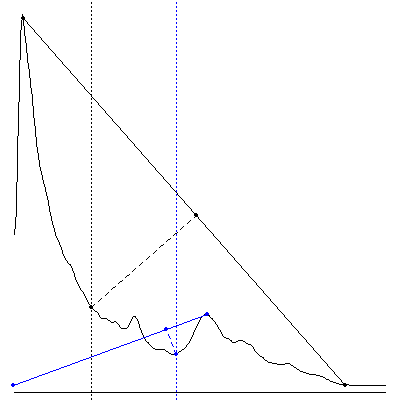 When
When diagnose = TRUE and adjust_par = TRUE, the function temporarily
adjusts margins to draw the geometric construction in a large square format
and restores the previous settings on exit. If adjust_par = FALSE, no
parameters are changed and the plot respects the current device/layout.
Value
A list with:
- lp
Lower peak DN.
- lc
Lower corner DN (Rosin on the left mode).
- tl
Low threshold derived from
lcanduc.- tm
Mid threshold derived from
lcanduc.- th
High threshold derived from
lcanduc.- uc
Upper corner DN (Rosin on the right mode).
- up
Upper peak DN.
References
Macfarlane C (2011).
“Classification method of mixed pixels does not affect canopy metrics from digital images of forest overstorey.”
Agricultural and Forest Meteorology, 151(7), 833–840.
doi:10.1016/j.agrformet.2011.01.019.
Rosin PL (2001).
“Unimodal thresholding.”
Pattern Recognition, 34(11), 2083–2096.
ISSN 0031-3203, doi:10.1016/s0031-3203(00)00136-9.
Examples
caim <- conventional_lens_image()
# Prominence-based peak detection, Gaussian smoothing with sigma = 2 DN
thr <- thr_twocorner(caim$Blue[], sigma = 2, slope_reduction = FALSE,
                     method = "prominence")
# Original Macfarlane peak search (for comparison)
thr2 <- thr_twocorner(caim$Blue[], sigma = 2, slope_reduction = TRUE,
                      method = "macfarlane")
data.frame(unlist(thr), unlist(thr2))
Validate CIE sky models
Description
Validate CIE sky models fitted with fit_cie_model() (or ootb_sky_cie())
using k-fold cross-validation on relative radiance.
Usage
validate_cie_model(model, k = 10)
Arguments
model |
list. Output of |
k |
numeric vector of length one. Number of folds. |
Details
Validation uses k-fold cross-validation with k = 10 by default
(Kohavi 1995). For each fold, predictions are
compared against observed relative radiance and a simple linear regression
of predicted vs. observed is fitted, following
Piñeiro et al. (2008). Outliers are detected with a
median–MAD rule (see rem_outliers()) using a threshold of 3
and removed before fitting the regression.
Value
A list with:
- lm
An object of class
lm(seestats::lm()) for predicted vs. observed.- pred
Numeric vector of predicted relative radiance used in
lm.- obs
Numeric vector of observed relative radiance used in
lm.- r_squared
Coefficient of determination (
R^2).- rmse
Root mean squared error (RMSE).
- mae
Median absolute error (MAE).
- is_outlier
Logical vector marking outliers (MAD > 3) in the original sky-point set.
- metric
Numeric value. Mean squared deviation as in Gauch et al. (2003).
References
Gauch HG, Hwang JTG, Fick GW (2003).
“Model evaluation by comparison of model‐based predictions and measured values.”
Agronomy Journal, 95(6), 1442–1446.
ISSN 1435-0645, doi:10.2134/agronj2003.1442.
Kohavi R (1995).
“A study of cross-validation and bootstrap for accuracy estimation and model selection.”
In Proceedings of the 14th International Joint Conference on Artificial Intelligence - Volume 2, IJCAI'95, 1137–1143.
ISBN 1558603638.
Piñeiro G, Perelman S, Guerschman JP, Paruelo JM (2008).
“How to evaluate models: Observed vs. predicted or predicted vs. observed?”
Ecological Modelling, 216(3-4), 316–322.
doi:10.1016/j.ecolmodel.2008.05.006.
Examples
## Not run:
caim <- read_caim()
z <- zenith_image(ncol(caim), lens())
a <- azimuth_image(z)
path <- system.file("external/sky_points.csv", package = "rcaiman")
sky_points <- read.csv(path)[c("Y", "X")]
names(sky_points) <- c("row", "col")
rr <- extract_rr(caim$Blue, z, a, sky_points)

set.seed(7)
model <- fit_cie_model(rr, sun_angles = c(z = 49.5, a = 27.4),
                       general_sky_type = "Clear", method = "CG")
val <- validate_cie_model(model, k = 10)
val$r_squared
val$rmse

## End(Not run)
Write canopy image
Description
Wrapper around terra::writeRaster() that writes a canopy image as GeoTIFF
with 8- or 16-bit unsigned integers, setting CRS and extent.
Usage
write_caim(caim, path, bit_depth)
Arguments
caim |
|
path |
character vector of length one. Destination file path (extension
|
bit_depth |
numeric vector of length one. Either |
Details
Adds the .tif extension to path if missing. The CRS is set to EPSG:7589
and the extent to [0, ncol] × [0, nrow] in pixel units. Data are written as
INT1U when bit_depth = 8 and INT2U when bit_depth = 16.
Value
No return value. Called for side effects.
Examples
## Not run:
caim <- read_caim() %>% normalize_minmax(0, 255)
write_caim(caim * (2^8 - 1),  file.path(tempdir(), "test_8bit"),  8)
write_caim(caim * (2^16 - 1), file.path(tempdir(), "test_16bit"), 16)
# Note: values are scaled by (2^bit_depth - 1) to avoid the maximum bin,
# which read_caim() might turn NA.

## End(Not run)
Write and read out-of-the-box CIE sky model and raster
Description
Persist and restore the out-of-the-box CIE sky model, its diagnostics, and
related rasters/points. The writer produces a human-readable .txt manifest
plus CSV and GeoPackage sidecar files. The reader reconstructs a list object
compatible with the out-of-the-box pipeline.
Usage
write_sky_cie(sky_cie, name)

read_sky_cie(name, r, z, a, refit_allowed = FALSE)
Arguments
sky_cie |
list. Object holding the fitted CIE model, diagnostics, and derived rasters, as produced by the out-of-the-box workflow. |
name |
character vector of length one. File base name without extension.
A path can be included, e.g., |
r |
numeric terra::SpatRaster of one layer. The canopy image
used in the out-of-the-box workflow (used by |
z |
terra::SpatRaster generated with |
a |
terra::SpatRaster generated with |
refit_allowed |
logical vector of length one. If |
Details
Encoding is UTF-8. Decimal point is .. Unknown keys are
ignored with a warning. Missing required keys trigger an error. The manifest
begins with format_version: which is checked for basic compatibility.
When read_sky_cie() detects manual edits (moved sun disk or changed sky
points) and refit_allowed = TRUE, it re-fits the CIE model using the
current r, z, and a, then revalidates.
Value
See Functions.
Functions
write_sky_cieNo return value. Writes six files to disk with the prefix
name(see below).read_sky_cieReturns a
listsimilar to the output ofootb_sky_cie()and suitable as input toootb_sky_above().
Files written by write_sky_cie
Plain text manifest:
name.txtCSV with sky radiance samples:
name_rr.csvCSV with sky radiance samples for the upward pass:
name_rr_up.csv(optional)GeoPackage with sky sample points:
name_sky_points.gpkgGeoPackage with the sun disk location:
name_sun_disk.gpkgCSV with validation pairs:
name_val.csv
Text file keys
format_version:Semantic version of the manifest.
sun_theta:Solar zenith (deg).
sun_phi:Solar azimuth (deg).
method_sun:Method used to optimize sun coordinates.
zenith_dn:Reference DN at zenith.
start_a:…start_e:Initial CIE coefficients.
is_from_detected_sky_dn:Enables
_rr_up.csvifTRUE.fit_a:…fit_e:Fitted CIE coefficients.
method:Method used to fit CIE coefficients.
dist_to_black:Argument passed to
extract_sky_points().grid:Sky grid parameters (
angle_width,first_ring_different).min_spherical_dist:Sampling buffer distance (deg).
sky_points_no:Number of sky points.
outliers_no:Number of sky points that were detected as outliers.
rmse:Validation metrics. Root mean squared error.
r_squared:Validation metric. Coefficient of determination.
mae:Validation metrics. Mean absolute error.
[Tested: …]Enumerates tested methods/grids/distances.
Examples
## Not run:
caim <- read_caim()
z <- zenith_image(ncol(caim), lens())
a <- azimuth_image(z)

# Read a previously written model
path <- system.file("external/example.txt", package = "rcaiman")
sky_cie <- read_sky_cie(gsub(".txt", "", path), r = caim$Blue, z = z, a = a,
                        refit_allowed = TRUE)

## End(Not run)
Map between zenith–azimuth angles and raster coordinates
Description
Bidirectional helpers to convert between angular coordinates on the
hemispherical image (zenith, azimuth) and raster
coordinates (row, col).
Usage
zenith_azimuth_from_row_col(z, a, row, col)

row_col_from_zenith_azimuth(z, a, zenith, azimuth)
Arguments
z |
terra::SpatRaster generated with |
a |
terra::SpatRaster generated with |
row, col |
numeric vectors. raster coodinates. Must have equal length. |
zenith, azimuth |
numeric vectors. Angles in degrees. Must have equal length. |
Details
zenith, azimuth → row, col.
A sparse set of valid sky points is sampled over the image and enriched with
their angular coordinates. Two local least-squares surfaces
(spatial::surf.ls, np = 6) are fitted to predict row and col as
smooth functions of (azimuth, zenith). Predictions are rounded to the
nearest integer index. Out-of-bounds indices are not produced under normal
conditions; clamp externally if needed.
row, col → zenith, azimuth.
Angles are obtained by direct lookup on z and a using
terra::cellFromRowCol. If any queried cell is NA (e.g., outside the
calibrated lens footprint), a synthetic z is reconstructed from the lens
model attached to z (attribute lens_coef), and a is rebuilt with
azimuth_image() using the stored orientation attribute in a. This yields
robust angle retrieval near borders.
Value
See Functions
Functions
row_col_from_zenith_azimuthReturn image indices for given angles.
zenith_azimuth_from_row_colReturn angles in degrees for given image indices.
Examples
z <- zenith_image(1000, lens())
a <- azimuth_image(z)

rc <- row_col_from_zenith_azimuth(z, a, zenith = c(30, 60), azimuth = c(90, 270))
rc

ang <- zenith_azimuth_from_row_col(z, a, row = rc$row, col = rc$col)
ang
Build Zenith image
Description
Build a single-layer image with zenith angle values, assuming upwards-looking hemispherical photography with the optical axis vertically aligned.
Usage
zenith_image(diameter, lens_coef)
Arguments
diameter |
numeric vector of length one. Diameter in pixels expressed as an even integer. This places the zenith point between pixels. Snapping the zenith point between pixels does not affect accuracy because half-pixel is less than the uncertainty in localizing the circle within the picture. |
lens_coef |
numeric vector. Polynomial coefficients of the lens
projection function. See |
Value
terra::SpatRaster with zenith angles in
degrees, showing a complete hemispherical view with the zenith at the
center. The object carries attributes lens_coef.
Examples
z <- zenith_image(600, lens("Nikon_FCE9"))
plot(z)