| Version: | 1.2-4 |
| Encoding: | UTF-8 |
| Date: | 2024-07-10 |
| Title: | Quantile-Based Spectral Analysis of Time Series |
| Depends: | R (≥ 3.0.0), stats4 |
| Suggests: | testthat |
| Imports: | methods, graphics, quantreg, abind, zoo, snowfall, Rcpp (≥ 0.11.0) |
| Description: | Methods to determine, smooth and plot quantile periodograms for univariate and multivariate time series. See Kley (2016) <doi:10.18637/jss.v070.i03> for a description and tutorial. |
| License: | GPL-2 | GPL-3 [expanded from: GPL (≥ 2)] |
| URL: | https://github.com/tobiaskley/quantspec |
| BugReports: | https://github.com/tobiaskley/quantspec/issues |
| LazyData: | TRUE |
| LinkingTo: | Rcpp |
| Collate: | 'Class-BootPos.R' 'generics.R' 'Class-LagOperator.R' 'Class-ClippedCov.R' 'Class-QSpecQuantity.R' 'aux-functions.R' 'Class-FreqRep.R' 'Class-ClippedFT.R' 'Class-QuantileSD.R' 'Class-IntegrQuantileSD.R' 'Class-Weight.R' 'Class-KernelWeight.R' 'Class-LagEstimator.R' 'kernels.R' 'Class-LagKernelWeight.R' 'Class-MovingBlocks.R' 'Class-QRegEstimator.R' 'Class-QuantilePG.R' 'Class-SmoothedPG.R' 'Class-SpecDistrWeight.R' 'RcppExports.R' 'data.R' 'deprecated.R' 'models.R' 'quantspec-package.R' |
| RoxygenNote: | 7.3.2 |
| NeedsCompilation: | yes |
| Packaged: | 2024-07-10 13:05:01 UTC; tkley |
| Author: | Tobias Kley [aut, cre], Stefan Birr [ctb] (Contributions to lag window estimation) |
| Maintainer: | Tobias Kley <tobias.kley@uni-goettingen.de> |
| Repository: | CRAN |
| Date/Publication: | 2024-07-11 12:50:02 UTC |
Quantile-Based Spectral Analysis of Time Series
Description
Methods to determine, smooth and plot quantile periodograms for univariate and (since v1.2-0) multivariate time series. See Kley (2016) <doi:10.18637/jss.v070.i03> for a description and tutorial.
Details
| Package: | quantspec |
| Type: | Package |
| Version: | 1.2-4 |
| Date: | 2024-07-10 |
| License: | GPL (>= 2) |
Contents
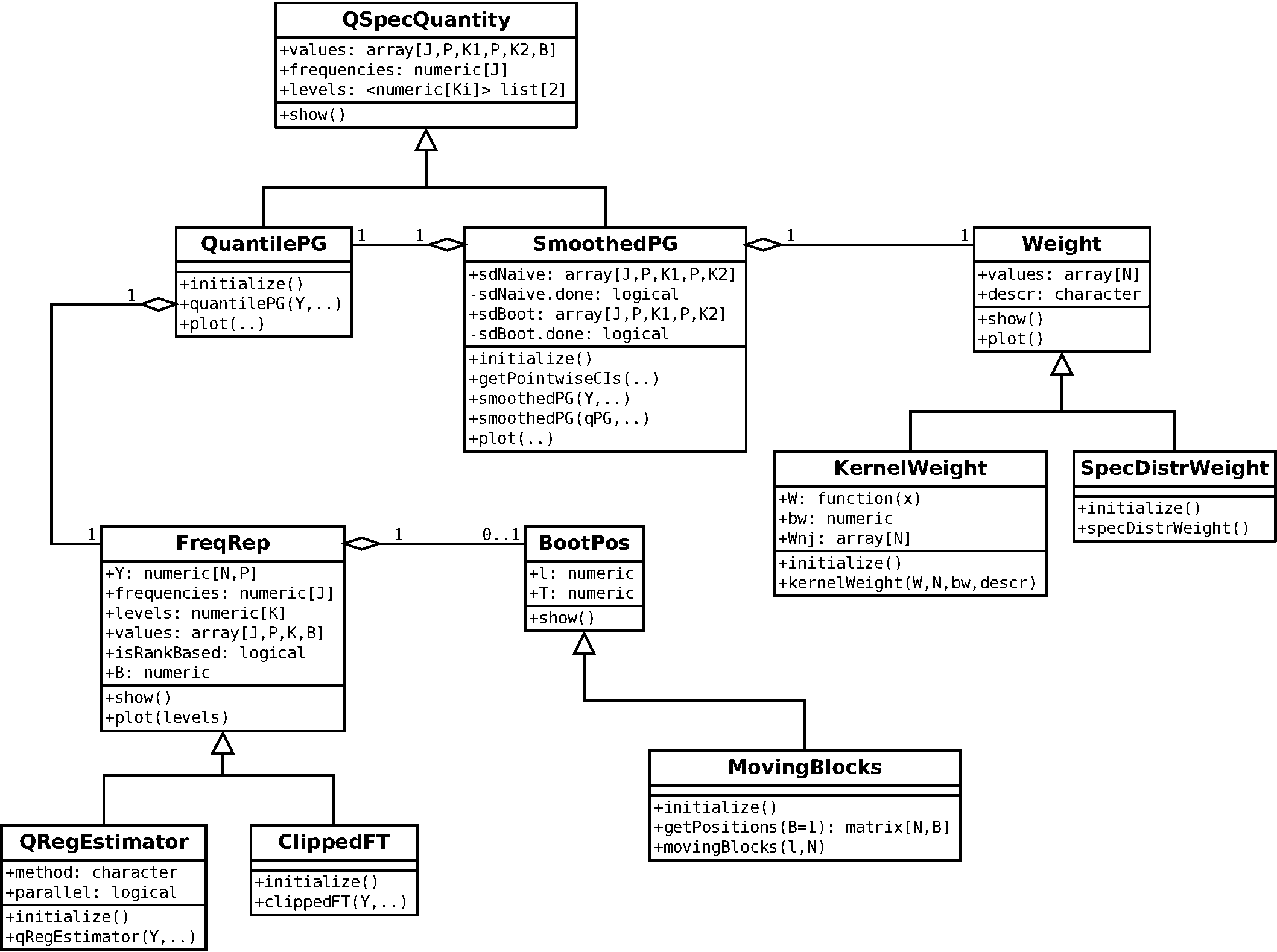
The quantspec package contains a hierachy of S4 classes with corresponding methods and functions serving as constructors. The following class diagrams provide an overview on the structure of the package. In the first and second class diagram the classes implementing the estimators are shown. In the first diagram the classes related to periodogram-based estimation are displayed:
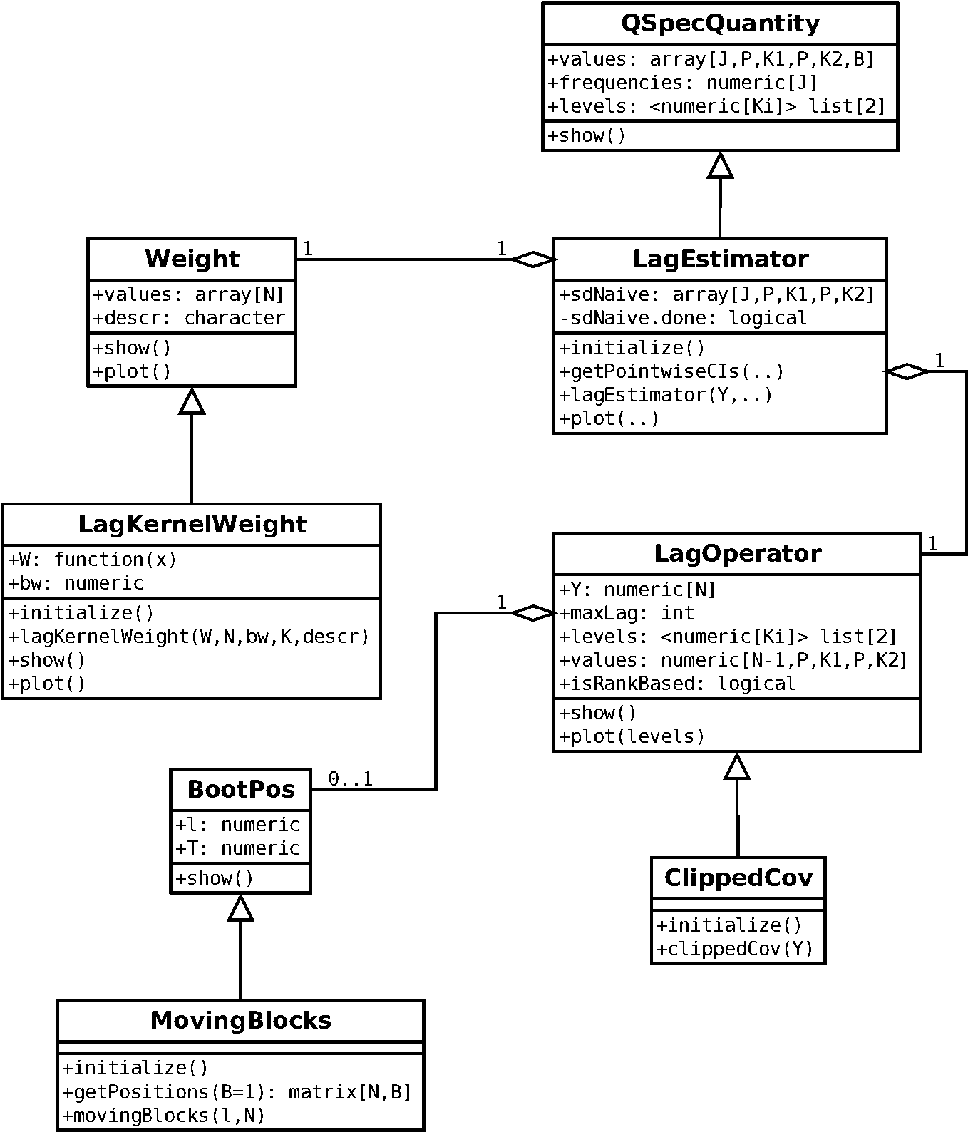
In the second diagram the classes related to lag window-based estimation are displayed:
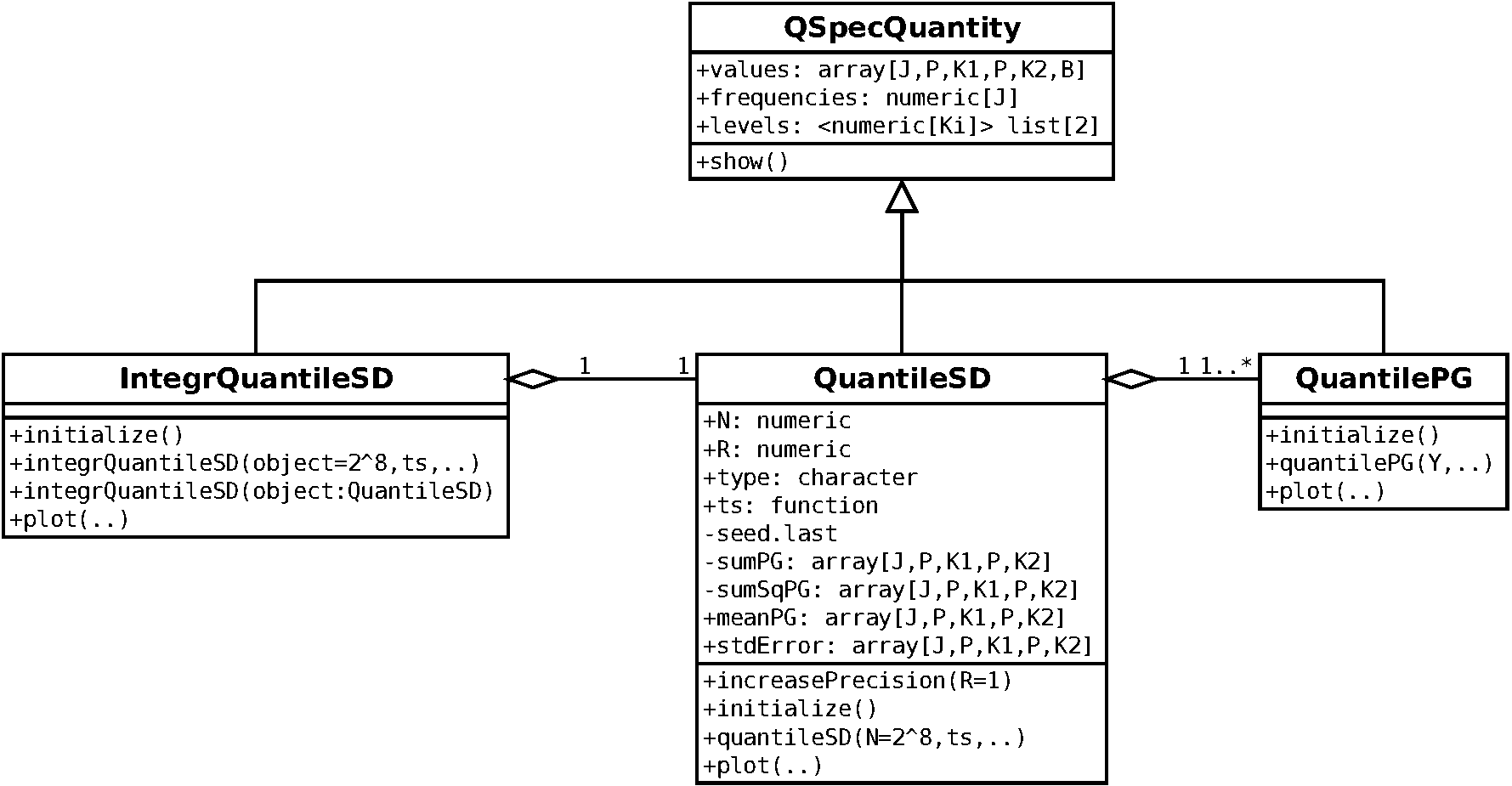
In the third class diagram the classes implementing model quantities are
displayed. A relation to the “empirical classes” is given via the fact that
the quantile spectral densities are computed by simulation of quantile
periodograms and a common abstract superclass QSpecQuantity which
is used to provide a common interface to quantile spectral quantities.
Besides the object-oriented design a few auxiliary functions exists. They serve as parameters or are mostly for internal use. A more detailed description of the framework can be found in the paper on the package (Kley, 2016).
Organization of the source code / files in the /R folder
All of the source code related to the specification of a certain class is
contained in a file named Class-[Name_of_the_class].R. This includes,
in the following order,
all roxygen
@includeto insure the correctly generated collate for the DESCRIPTION file.-
\setClasspreceded by a meaningful roxygen documentation. specification of an
initializemethod, where appropriate.all accessor and mutator method (i. e., getter and setter); first the ones returning attributes of the object, then the ones returning associated objects.
constructors; use generics if there is more than one of them.
-
showandplotmethods.
Coding Conventions
To improve readability of the software and documentation this package was written in the spirit of the “Coding conventions of the Java Programming Language” (Oracle, 2015). In particular, the naming conventions for classes and methods have been adopted, where “Class names should be nouns, in mixed case with the first letter of each internal word capitalized.” and “Methods should be verbs, in mixed case with the first letter lowercase, with the first letter of each internal word capitalized.”
Naming Conventions for the Documentation
To reflect the structure of the contents of the package in the documentation file, the following system for naming of the sections is adopted:
Documentation of an S4 class is named as the name of the class followed by “-class”. [cf.
QuantilePG-class]Documentation of a constructor for an S4-class is named as the name of the class followed by “-constructor”. [cf.
QuantilePG-constructor]Documentation of a method dispaching to an object of a certain S4 class is named by the name of the method, followed by “-”, followed by the name of the Class. [cf.
getValues-QuantilePG]
Author(s)
Tobias Kley
References
Kley, T. (2014a). Quantile-Based Spectral Analysis: Asymptotic Theory and Computation. Ph.D. Dissertation, Ruhr University Bochum. https://hss-opus.ub.ruhr-uni-bochum.de/opus4/frontdoor/index/index/docId/3894.
Kley, T. (2016). Quantile-Based Spectral Analysis in an Object-Oriented Framework and a Reference Implementation in R: The quantspec Package. Journal of Statistical Software, 70(3), 1–27.
Dette, H., Hallin, M., Kley, T. & Volgushev, S. (2015).
Of Copulas, Quantiles, Ranks and Spectra: an L_1-approach to
spectral analysis. Bernoulli, 21(2), 781–831.
[cf. http://arxiv.org/abs/1111.7205]
Kley, T., Volgushev, S., Dette, H. & Hallin, M. (2016). Quantile Spectral Processes: Asymptotic Analysis and Inference. Bernoulli, 22(3), 1770–1807. [cf. http://arxiv.org/abs/1401.8104]
Barunik, J. & Kley, T. (2019). Quantile Coherency: A General Measure for Dependence between Cyclical Economic Variables. Econometrics Journal, 22, 131–152. [cf. http://arxiv.org/abs/1510.06946]
Oracle (2015). Coding conventions of the Java Programming Language. https://www.oracle.com/java/technologies/javase/codeconventions-contents.html. Accessed 2015-03-25.
See Also
Useful links:
Report bugs at https://github.com/tobiaskley/quantspec/issues
Workhorse function for getCoherency-SmoothedPG.
Description
C++ implementation to increase performance.
Arguments
V |
a 3-dimensional array of complex numbers; dimensions are
|
W |
a vector of length |
Value
Returns an array with complex numbers
\sigma(\tau_1, \tau_2, \omega_j as defined in
Kley et. al (2016), p. 26.
References
Barunik, J. & Kley, T. (2019). Quantile Coherency: A General Measure for Dependence Between Cyclical Economic Variables. Econometrics Journal, 22, 131–152. http://arxiv.org/abs/1401.8104.
Workhorse function for getSdNaive-SmoothedPG.
Description
C++ implementation to increase performance.
Arguments
V |
a 3-dimensional array of complex numbers; dimensions are
|
W |
a vector of length |
Value
Returns an array with complex numbers
\sigma(\tau_1, \tau_2, \omega_j as defined in
Kley et. al (2016), p. 26.
References
Dette, H., Hallin, M., Kley, T. & Volgushev, S. (2015).
Of Copulas, Quantiles, Ranks and Spectra: an L_1-approach to
spectral analysis. Bernoulli, 21(2), 781–831.
[cf. http://arxiv.org/abs/1111.7205]
Class for Generation of Bootstrapped Replications of a Time Series.
Description
BootPos is an S4 class that provides a common interface
to different algorithms that can be used for implementation of a block
bootstrap procedure in the time domain.
Details
After initialization the bootstrapping can be performed by applying
getPositions to the object.
Different block bootstraps are implemented by creating a subclass together
with a getPositions method that contains the implementation of the
block resampling procedure.
Currently the following implementations are available:
Slots
lthe (expected) block length for the block bootstrap methods
Nnumber of available observations to bootstrap from
References
Lahiri, S. N. (1999). Theoretical Comparisons of Block Bootstrap Methods. The Annals of Statistics, 27(1), 386–404.
Class to calculate copula covariances from a time series with given levels.
Calculates for each combination of levels (\tau_1,\tau_2)
and for all k < \code{maxLag} the copula covariances
Cov(1_{X_0 < \tau_1},1_{X_k < \tau_2})
and writes it to values[k] from its superclass LagOperator.
Description
For each lag k = 0, ..., maxLag and combination of levels
(\tau_1, \tau_2) from levels.1 x levels.2 the
statistic
\frac{1}{n} \sum_{t=1}^{n-k} ( I\{\hat F_n(Y_t) \leq \tau_1\} - \tau_1) ( I\{\hat F_n(Y_{t+k}) \leq \tau_2\} - \tau_2)
is determined and stored to the array values.
Details
Currently, the implementation of this class allows only for the analysis of univariate time series.
Create an instance of the ClippedCov class.
Description
Create an instance of the ClippedCov class.
Usage
clippedCov(
  Y,
  maxLag = length(Y) - 1,
  levels.1 = c(0.5),
  levels.2 = levels.1,
  isRankBased = TRUE,
  B = 0,
  l = 0,
  type.boot = c("none", "mbb")
)
Arguments
Y |
Time series to calculate the copula covariance from |
maxLag |
maximum lag between observations that should be used |
levels.1 |
a vector of numerics that determines the level of clipping |
levels.2 |
a vector of numerics that determines the level of clipping |
isRankBased |
If true the time series is first transformed to pseudo data; currently only rank-based estimation is possible. |
B |
number of bootstrap replications |
l |
(expected) length of blocks |
type.boot |
A flag to choose a method for the block bootstrap; currently
two options are implemented: |
Value
Returns an instance of ClippedCov.
See Also
Examples
ccf <- clippedCov(rnorm(200), maxLag = 25, levels.1 = c(0.1,0.5,0.9))
dim(getValues(ccf))
#print values for levels (.5,.5)
plot(ccf, maxLag = 20)
Class for Fourier transform of the clipped time series.
Description
ClippedFT is an S4 class that implements the necessary
calculations to determine the Fourier transform of the clipped time
series. As a subclass to FreqRep it inherits
slots and methods defined there; it servers as a frequency representation of
a time series as described in Kley et. al (2016) for univariate time series
and in Barunik & Kley (2015) for multivariate time series.
Details
For each frequency \omega from frequencies and level q
from levels the statistic
\sum_{t=0}^{n-1} I\{Y_{t,i} \leq q\} \mbox{e}^{-\mbox{i} \omega t}
is determined and stored to the array values. Internally the methods
mvfft and fft are used to achieve
good performance.
Note that, all remarks made in the documentation of the super-class
FreqRep apply.
References
Kley, T., Volgushev, S., Dette, H. & Hallin, M. (2016). Quantile Spectral Processes: Asymptotic Analysis and Inference. Bernoulli, 22(3), 1770–1807. [cf. http://arxiv.org/abs/1401.8104]
Barunik, J. & Kley, T. (2015). Quantile Cross-Spectral Measures of Dependence between Economic Variables. [preprint available from the authors]
See Also
For an example see FreqRep.
Create an instance of the ClippedFT class.
Description
The parameter type.boot can be set to choose a block bootstrapping
procedure. If "none" is chosen, a moving blocks bootstrap with
l=lenTS(Y) and N=lenTS(Y) would be done. Note that in that
case one would also chose B=0 which means that getPositions
would never be called. If B>0 then each bootstrap replication would
be the undisturbed time series.
Usage
clippedFT(
  Y,
  frequencies = 2 * pi/lenTS(Y) * 0:(lenTS(Y) - 1),
  levels = 0.5,
  isRankBased = TRUE,
  B = 0,
  l = 0,
  type.boot = c("none", "mbb")
)
Arguments
Y |
A |
frequencies |
A vector containing frequencies at which to determine the quantile periodogram. |
levels |
A vector of length |
isRankBased |
If true the time series is first transformed to pseudo
data [cf. |
B |
number of bootstrap replications |
l |
(expected) length of blocks |
type.boot |
A flag to choose a method for the block bootstrap; currently
two options are implemented: |
Value
Returns an instance of ClippedFT.
See Also
For an example see FreqRep.
Class for Frequency Representation.
Description
FreqRep is an S4 class that encapsulates, for a multivariate time
series (Y_{t,i})_{t=0,\ldots,n-1},
i=1,\ldots,d
the data structures for the storage of a frequency representation. Examples
of such frequency representations include
the Fourier transformation of the clipped time series
(\{I\{Y_{t,i} \leq q\}), orthe weighted
L_1-projection of(Y_{t,i})onto an harmonic basis.
Examples are realized by implementing a sub-class to
FreqRep.
Currently, implementations for the two examples mentioned above are available:
ClippedFT and
QRegEstimator.
Details
It is always an option to base the calculations on the pseudo data
R_{t,n,i} / n where R_{t,n,i} denotes the rank of
Y_{t,i} among (Y_{t,i})_{t=0,\ldots,n-1}.
To allow for a block bootstrapping procedure a number of B estimates
determined from bootstrap replications of the time series which are yield by
use of a BootPos-object can be stored on initialization.
The data in the frequency domain is stored in the array values, which
has dimensions (J,P,K,B+1), where J is the number of
frequencies, P is the dimension of the time series,
K is the number of levels and B is
the number of bootstrap replications requested on intialization.
In particular, values[j,i,k,1] corresponds to the time series' frequency
representation with frequencies[j], dimension i and levels[k], while
values[j,i,k,b+1] is the for the same, but determined from the
bth block bootstrapped replicate of the time series.
Slots
YThe time series of which the frequency representation is to be determined.
frequenciesThe frequencies for which the frequency representation will be determined. On initalization
frequenciesValidatoris called, so that it will always be a vector of reals from[0,\pi]. Also, only Fourier frequencies of the form2\pi j / nwith integersjandnthelength(Y)are allowed.levelsThe levels for which the frequency representation will be determined. If the flag
isRankBasedis set toFALSE, then it can be any vector of reals. IfisRankBasedis set toTRUE, then it has to be from[0,1].valuesThe array holding the determined frequency representation. Use a
getValuesmethod of the relevant subclass to access it.isRankBasedA flag that is
FALSEif the determinedvaluesare based on the original time series andTRUEif it is based on the pseudo data as described in the Details section of this topic.positions.bootAn object of type
BootPos, that is used to determine the block bootstrapped replicates of the time series.BNumber of bootstrap replications to perform.
Examples
Y       <- rnorm(32)
freq    <- 2*pi*c(0:31)/32
levels  <- c(0.25,0.5,0.75)
cFT     <- clippedFT(Y, freq, levels)

plot(cFT)

# Get values for all Fourier frequencies and all levels available.
V.all    <- getValues(cFT)

# Get values for every second frequency available
V.coarse <- getValues(cFT, frequencies = 2*pi*c(0:15)/16, levels = levels)

# Trying to get values on a finer grid of frequencies than available will
# yield a warning and then all values with frequencies closest to that finer
# grid.
V.fine   <- getValues(cFT, frequencies = 2*pi*c(0:63)/64, levels = levels)

# Finally, get values for the available Fourier frequencies from [0,pi] and
# only for tau=0.25
V.part   <- getValues(cFT, frequencies = 2*pi*c(0:16)/32, levels = c(0.25))

# Alternatively this can be phrased like this:
V.part.alt <- getValues(cFT, frequencies = freq[freq <= pi], levels = c(0.25))
Class for a simulated integrated quantile (i. e., Laplace or copula) density kernel.
Description
IntegrQuantileSD is an S4 class that implements the necessary
calculations to determine an integrated version of the quantile spectral
density kernel (computed via QuantileSD).
In particular it can be determined for any model from which a time series
of length N can be sampled via a function call ts(N).
Details
In the simulation the quantile spectral density is first determined via
QuantileSD, it's values are recovered using
getValues-QuantileSD and then cumulated using cumsum.
Note that, all remarks made in the documentation of the super-class
QSpecQuantity apply.
Slots
qsda
QuantileSDfrom which to begin the computations.
Examples
################################################################################
## This script illustrates how to estimate integrated quantile spectral densities

## Simulate a time series Y1,...,Y128 from the QAR(1) process discussed in
## Dette et. al (2015).
set.seed(2581)
Y <- ts1(128)

## For a defined set of quantile levels ...
levels <- c(0.25,0.5,0.75)

## ... and a weight (of Type A), defined using the Epanechnikov kernel ...
wgt <- specDistrWeight()

## ... compute a smoothed quantile periodogram (based on the clipped time series).
## Repeat the estimation 100 times, using the moving blocks bootstrap with
## block length l=32.
sPG.cl <- smoothedPG(Y, levels.1 = levels, type="clipped", weight = wgt,
    type.boot = "mbb", B=100, l=32)

## Create a (model) spectral density kernel for he QAR(1) model for display
## in the next plot.
csd <- quantileSD(N=2^8, seed.init = 2581, type = "copula",
    ts = ts1, levels.1=levels, R = 100)
icsd <- integrQuantileSD(csd)

plot(sPG.cl, ptw.CIs = 0.1, qsd = icsd, type.CIs = "boot.full")
Create an instance of the IntegrQuantileSD class.
Description
Create an instance of the IntegrQuantileSD class.
Usage
integrQuantileSD(
  object = 2^8,
  type = c("copula", "Laplace"),
  ts = rnorm,
  seed.init = 2581,
  levels.1 = 0.5,
  levels.2 = levels.1,
  R = 1,
  quiet = FALSE
)
Arguments
object |
the number |
type |
can be either |
ts |
a function that has one argument |
seed.init |
an integer serving as an initial seed for the simulations. |
levels.1 |
A vector of length |
levels.2 |
A vector of length |
R |
an integer that determines the number of independent simulations; the larger this number the more precise is the result. |
quiet |
Don't report progress to console when computing the |
Value
Returns an instance of IntegrQuantileSD.
See Also
For an example see IntegrQuantileSD.
Class for Brillinger-type Kernel weights.
Description
KernelWeight is an S4 class that implements a weighting function by
specification of a kernel function W and a scale parameter bw.
Details
It extends the class Weight and writes
W_N(2\pi (k-1)/N) := \sum_{j \in Z} bw^{-1} W(2\pi bw^{-1} [(k-1)/N + j])
to values[k] [nested inside env] for k=1,...,N.
The number length(values) of Fourier frequencies for which
W_N will be evaluated may be set on construction or updated when
evoking the method getValues.
To standardize the weights used in the convolution to unity
W_N^j := \sum_{j \neq s = 0}^{N-1} W_n(2\pi s / N)
is stored to Wnj[s] for s=1,...,N, for later usage.
Slots
Wa kernel function
bwbandwidth
envAn environment to allow for slots which need to be accessable in a call-by-reference manner:
valuesA vector storing the weights; see the Details section.
WnjA vector storing the terms used for normalization; see the Details section.
References
Brillinger, D. R. (1975). Time Series: Data Analysis and Theory. Holt, Rinehart and Winston, Inc., New York. [cf. p. 146 f.]
See Also
Examples for implementations of kernels W can be found at:
kernels.
Create an instance of the KernelWeight class.
Description
Create an instance of the KernelWeight class.
Usage
kernelWeight(
  W = W0,
  N = 1,
  bw = 0.1 * N^(-1/5),
  descr = paste("bw=", round(bw, 3), ", N=", N, sep = "")
)
Arguments
W |
A kernel function |
N |
Fourier basis; number of grid points in |
bw |
bandwidth; if a vector, then a list of weights is returned |
descr |
a description to be used in some plots |
Value
Returns an instance of KernelWeight.
See Also
Examples
wgt1 <- kernelWeight(W=W0, N=16, bw=c(0.1,0.3,0.7))
print(wgt1)
wgt2 <- kernelWeight(W=W1, N=2^8, bw=0.1)
plot(wgt2, main="Weights determined from Epanechnikov kernel")
Class for a lag-window type estimator.
Description
For a given time series Y a lag-window estimator of the Form
\hat{f}(\omega) = \sum_{|k|< n-1 } K_n(k) \Gamma(Y_0,Y_k) \exp(-i \omega k)
will be calculated on initalization. The LagKernelWeight K_n is determined
by the slot weight and the LagOperator \Gamma(Y_0,Y_k) is defined
by the slot lagOp.
Details
Currently, the implementation of this class allows only for the analysis of univariate time series.
Slots
Ythe time series where the lag estimator was applied one
weighta
Weightobject to be used as lag windowlagOpa
LagOperatorobject that determines which kind of bivariate structure should be calculated.envAn environment to allow for slots which need to be accessable in a call-by-reference manner:
sdNaiveAn array used for storage of the naively estimated standard deviations of the smoothed periodogram.
sdNaive.donea flag indicating whether
sdNaivehas been set yet.
Create an instance of the LagEstimator class.
Description
A LagEstimator object can be created from numeric, a ts,
or a zoo object. Also a LagOperator and a
Weight object can be used to create different types of
estimators.
Usage
lagEstimator(
  Y,
  frequencies = 2 * pi/length(Y) * 0:(length(Y) - 1),
  levels.1 = 0.5,
  levels.2 = levels.1,
  weight = lagKernelWeight(K = length(Y), bw = 100),
  type = c("clippedCov")
)
Arguments
Y |
a time series ( |
frequencies |
A vector containing (Fourier-)frequencies at which to determine the smoothed periodogram. |
levels.1 |
the first vector of levels for which to compute the LagEstimator |
levels.2 |
the second vector of levels for which to compute the LagEstimator |
weight |
Object of type |
type |
if |
Value
Returns an instance of LagEstimator.
Examples
Y <- rnorm(100)
levels.1 <- c(0.1,0.5,0.9)
weight <- lagKernelWeight(W = WParzen,  bw = 10, K = length(Y))
lagOp <- clippedCov(Y,levels.1 = levels.1)
lagEst <- lagEstimator(lagOp, weight = weight)
Class for lag window generators
Description
LagKernelWeight is an S4 class that implements a weighting function by
specification of a kernel function W and a scale parameter bw.
Details
It extends the class Weight and writes
W_N(x[k]) := W(x[k]/bw)
to values[k] [nested inside env] for k=1,...,length(x).
The points x where W is evaluated may be set on construction or updated when
evoking the method getValues.
Slots
Wa kernel function
bwbandwidth
envAn environment to allow for slots which need to be accessable in a call-by-reference manner:
valuesA vector storing the weights; see the Details section.
See Also
Examples for implementations of kernels W can be found at:
kernels.
Create an instance of the LagKernelWeight class.
Description
Create an instance of the LagKernelWeight class.
Usage
lagKernelWeight(
  W = WParzen,
  bw = K/2,
  K = 10,
  descr = paste("bw=", bw, ", K=", K, sep = "")
)
Arguments
W |
A kernel function |
bw |
bandwidth |
K |
a |
descr |
a description to be used in some plots |
Value
Returns an instance of LagKernelWeight.
See Also
Examples
wgt1 <- lagKernelWeight(W=WParzen, K=20, bw=10)
print(wgt1)
Interface Class to access different types of operators on time series.
Description
LagOperator is an S4 class that provides a common interface to
implementations of an operator \Gamma(Y) which is calculated on
all pairs of observations (Y_0,Y_k) with lag smaller than maxLag
Details
Currently one implementation is available:
(1) ClippedCov.
Currently, the implementation of this class allows only for the analysis of univariate time series.
Slots
valuesan array of dimension
c(maxLag,length(levels.1),length(levels.2))containing the values of the operator.Yis the time series the operator shall be applied to
maxLagmaximum lag between two observations
levelsa vector of numerics that determines the levels of the operator
isRankBasedA flag that is
FALSEif the determinedvaluesare based on the original time series andTRUEif it is based on the ranks.positions.bootAn object of type
BootPos, that is used to determine the block bootstrapped replicates of the time series.BNumber of bootstrap replications to perform.
Class for Moving Blocks Bootstrap implementation.
Description
MovingBlocks is an S4 class that implements the moving blocks
bootstrap described in Künsch (1989).
Details
MovingBlocks extends the S4 class
BootPos and the remarks made in its documentation
apply here as well.
The Moving Blocks Bootstrap method of Künsch (1989) resamples blocks
randomly, with replacement from the collection of overlapping blocks of
length l that start with observation 1, 2, ..., N-l+1.
A more precise description of the procedure can also be found in
Lahiri (1999), p. 389.
References
Künsch, H. R. (1989). The jackknife and the bootstrap for general stationary observations. The Annals of Statistics, 17, 1217–1261.
See Also
Create an instance of the MovingBlocks class.
Description
Create an instance of the MovingBlocks class.
Usage
movingBlocks(l, N)
Arguments
l |
the block length for the block bootstrap methods |
N |
number of available observations to bootstrap from |
Value
Returns an instance of MovingBlocks.
Class for quantile regression-based estimates in the harmonic linear model.
Description
QRegEstimator is an S4 class that implements the necessary
calculations to determine the frequency representation based on the weigthed
L_1-projection of a time series as described in
Dette et. al (2015). As a subclass to FreqRep
it inherits slots and methods defined there.
Details
For each frequency \omega from frequencies and level
\tau from levels the statistic
\hat b^{\tau}_n(\omega) := \arg\max_{a \in R, b \in C}
      \sum_{t=0}^{n-1}
      \rho_{\tau}(Y_t - a - Re(b) \cos(\omega t) - Im(b) \sin(\omega t)),
is determined and stored to the array values.
The solution to the minimization problem is determined using the function
rq from the quantreg package.
All remarks made in the documentation of the super-class
FreqRep apply.
Slots
methodmethod used for computing the quantile regression estimates. The choice is passed to
qr; see the documentation ofquantregfor details.parallela flag that signalizes that parallelization mechanisms from the package snowfall may be used.
References
Dette, H., Hallin, M., Kley, T. & Volgushev, S. (2015).
Of Copulas, Quantiles, Ranks and Spectra: an L_1-approach to
spectral analysis. Bernoulli, 21(2), 781–831.
[cf. http://arxiv.org/abs/1111.7205]
Create an instance of the QRegEstimator class.
Description
The parameter type.boot can be set to choose a block bootstrapping
procedure. If "none" is chosen, a moving blocks bootstrap with
l=length(Y) and N=length(Y) would be done. Note that in that
case one would also chose B=0 which means that getPositions
would never be called. If B>0 then each bootstrap replication would
be the undisturbed time series.
Usage
qRegEstimator(
  Y,
  frequencies = 2 * pi/lenTS(Y) * 0:(lenTS(Y) - 1),
  levels = 0.5,
  isRankBased = TRUE,
  B = 0,
  l = 0,
  type.boot = c("none", "mbb"),
  method = c("br", "fn", "pfn", "fnc", "lasso", "scad"),
  parallel = FALSE
)
Arguments
Y |
A |
frequencies |
A vector containing frequencies at which to determine the
|
levels |
A vector of length |
isRankBased |
If true the time series is first transformed to pseudo
data [cf. |
B |
number of bootstrap replications |
l |
(expected) length of blocks |
type.boot |
A flag to choose a method for the block bootstrap; currently
two options are implemented: |
method |
method used for computing the quantile regression estimates.
The choice is passed to |
parallel |
a flag to allow performing parallel computations. |
Value
Returns an instance of QRegEstimator.
Examples
library(snowfall)

Y <- rnorm(100) # Try 2000 and parallel computation will in fact be faster.

# Compute without using snowfall capabilities
system.time(
  qRegEst1 <- qRegEstimator(Y, levels=seq(0.25,0.75,0.25), method="fn", parallel=FALSE)
)

# Set up snowfall
sfInit(parallel=TRUE, cpus=2, type="SOCK")
sfLibrary(quantreg)
sfExportAll()

# Compare how much faster the computation is when done in parallel
system.time(
  qRegEst2 <- qRegEstimator(Y, levels=seq(0.25,0.75,0.25), method="fn", parallel=TRUE)
)

sfStop()

# Compare results
V1 <- getValues(qRegEst1)
V2 <- getValues(qRegEst2)
sum(abs(V1-V2)) # Returns: [1] 0
Class for a Quantile Spectral Estimator.
Description
QSpecQuantity is an S4 class that provides a common interface to
objects that are of the functional form
f^{j_1, j_2}(\omega; x_1, x_2),
where j_1, j_2 are indices denoting components of a time series
or process, \omega is a frequency parameter and
x_1, x_2 are level parameters. For each combination of
parameters a complex number can be stored.
Examples for objects of this kind currently include the quantile (i. e.,
Laplace or copula) spectral
density kernel [cf. QuantileSD for an implementation], an
integrated version of the quantile spectral density kernels
[cf. IntegrQuantileSD for an implementation], and
estimators of it [cf. QuantilePG and SmoothedPG
for implementations].
Slots
valuesThe array holding the values
f^{j_1, j_2}(\omega; x_1, x_2).frequenciesThe frequencies
\omegafor which the values are available.levelsA list of vectors containing the levels
x_iserving as argument for the estimator.
Class for a quantile (i. e., Laplace or copula) periodogram.
Description
QuantilePG is an S4 class that implements the necessary
calculations to determine one of the periodogram-like statistics defined in
Dette et. al (2015) and Kley et. al (2016).
Details
Performs all the calculations to determine a quantile periodogram from a
FreqRep object upon initizalization (and on request
stores the values for faster access).
The two methods available for the estimation are the ones implemented as
subclasses of FreqRep:
the Fourier transformation of the clipped time series
(\{I\{Y_t \leq q\})[cf.ClippedFT], orthe weighted
L_1-projection of(Y_t)onto an harmonic basis [cf.QRegEstimator].
All remarks made in the documentation of the super-class
QSpecQuantity apply.
Slots
freqRepa
FreqRepobject where the quantile periodogram will be based on.
References
Dette, H., Hallin, M., Kley, T. & Volgushev, S. (2015).
Of Copulas, Quantiles, Ranks and Spectra: an L_1-approach to
spectral analysis. Bernoulli, 21(2), 781–831.
[cf. http://arxiv.org/abs/1111.7205]
Kley, T., Volgushev, S., Dette, H. & Hallin, M. (2016). Quantile Spectral Processes: Asymptotic Analysis and Inference. Bernoulli, 22(3), 1770–1807. [cf. http://arxiv.org/abs/1401.8104]
Examples
################################################################################
## This script illustrates how to work with QuantilePG objects

## Simulate a time series Y1,...,Y128 from the QAR(1) process discussed in
## Dette et. al (2015).
Y <- ts1(64)

## For a defined set of quantile levels
levels <- c(0.25,0.5,0.75)

## the various quantile periodograms can be calculated calling quantilePG:

## For a copula periodogram as in Dette et. al (2015) the option 'type="qr"'
## has to be used:
system.time(
    qPG.qr <- quantilePG(Y, levels.1 = levels, type="qr"))

## For the CR-periodogram as in Kley et. al (2016) the option 'type="clipped"'
## has to be used. If bootstrap estimates are to be used the parameters
## type.boot, B and l need to be specified.
system.time(
    qPG.cl <- quantilePG(Y, levels.1 = levels, type="clipped",
        type.boot="mbb", B=250, l=2^5))

## The two previous calls also illustrate that computation of the CR-periodogram
## is much more efficient than the quantile-regression based copula periodogram.

## Either periodogram can be plotted using the plot command
plot(qPG.cl)
plot(qPG.qr)

## Because the indicators are not centered it is often desired to exclude the
## frequency 0; further more the frequencies (pi,2pi) are not wanted to be
## included in the plot, because f(w) = Conj(f(2 pi - w)).
## Using the plot command it is possible to select frequencies and levels for
## the diagram:
plot(qPG.cl, frequencies=2*pi*(1:32)/64, levels=c(0.25))

## We can also plot the same plot together with a (simulated) quantile spectral
## density kernel
csd <- quantileSD(N=2^8, seed.init = 2581, type = "copula",
    ts = ts1, levels.1=c(0.25), R = 100)
plot(qPG.cl, qsd = csd, frequencies=2*pi*(1:32)/64, levels=c(0.25))

## Calling the getValues method allows for comparing the two quantile
## periodograms; here in a diagram:
freq <- 2*pi*(1:31)/32
V.cl <- getValues(qPG.cl, frequencies = freq, levels.1=c(0.25))
V.qr <- getValues(qPG.qr, frequencies = freq, levels.1=c(0.25))
plot(x = freq/(2*pi), Re(V.cl[,1,1,1]), type="l",
        ylab="real part -- quantile PGs", xlab=expression(omega/2*pi))
lines(x = freq/(2*pi), Re(V.qr[,1,1,1]), col="red")

## Now plot the imaginary parts of the quantile spectra for tau1 = 0.25
## and tau2 = 0.5
freq <- 2*pi*(1:31)/32
V.cl <- getValues(qPG.cl, frequencies = freq, levels.1=c(0.25, 0.5))
V.qr <- getValues(qPG.qr, frequencies = freq, levels.1=c(0.25, 0.5))
plot(x = freq/(2*pi), Im(V.cl[,1,2,1]), type="l",
    ylab="imaginary part -- quantile PGs", xlab=expression(omega/2*pi))
lines(x = freq/(2*pi), Im(V.qr[,1,2,1]), col="red")
Create an instance of the QuantilePG class.
Description
The parameter type.boot can be set to choose a block bootstrapping
procedure. If "none" is chosen, a moving blocks bootstrap with
l=length(Y) and N=length(Y) would be done. Note that in that
case one would also chose B=0 which means that getPositions
would never be called. If B>0 then each bootstrap replication would
be the undisturbed time series.
Usage
quantilePG(
  Y,
  frequencies = 2 * pi/lenTS(Y) * 0:(lenTS(Y) - 1),
  levels.1 = 0.5,
  levels.2 = levels.1,
  isRankBased = TRUE,
  type = c("clipped", "qr"),
  type.boot = c("none", "mbb"),
  B = 0,
  l = 0,
  method = c("br", "fn", "pfn", "fnc", "lasso", "scad"),
  parallel = FALSE
)
Arguments
Y |
A |
frequencies |
A vector containing frequencies at which to determine the quantile periodogram. |
levels.1 |
A vector of length |
levels.2 |
A vector of length |
isRankBased |
If true the time series is first transformed to pseudo
data [cf. |
type |
A flag to choose the type of the estimator. Can be either
|
type.boot |
A flag to choose a method for the block bootstrap; currently
two options are implemented: |
B |
number of bootstrap replications |
l |
(expected) length of blocks |
method |
method used for computing the quantile regression estimates.
The choice is passed to |
parallel |
a flag to allow performing parallel computations, where possible. |
Value
Returns an instance of QuantilePG.
Class for a simulated quantile (i. e., Laplace or copula) density kernel.
Description
QuantileSD is an S4 class that implements the necessary
calculations to determine a numeric approximation to the quantile spectral
density kernel of a model from which a time series of length N can be
sampled via a function call ts(N).
Details
In the simulation a number of R independent quantile periodograms
based on the clipped time series are simulated. If type=="copula",
then the rank-based version is used. The sum and the sum of the squared
absolute value is stored to the slots sumPG and sumSqPG.
After the simulation is completed the mean and it's standard error (of the
simulated quantile periodograms) are determined and stored to meanPG
and stdError. Finally, the (copula) spectral density kernel is
determined by smoothing real and imaginary part of meanPG seperately
for each combination of levels using smooth.spline.
Note that, all remarks made in the documentation of the super-class
QSpecQuantity apply.
Slots
Na
numericspecifying the number of equaly spaced Fourier frequencies from[0,2\pi)for which the (copula) spectral density will be simulated; note that due to the simulation mechanism a larger number will also yield a better approximation.Rthe number of independent repetitions performed; note that due to the simulation mechanism a larger number will also yield a better approximation; can be enlarged using
increasePrecision-QuantileSD.typecan be either
Laplaceorcopula; indicates whether the marginals are to be assumed uniform[0,1]distributed.tsa
functionthat allows to draw independent samplesY_0, \ldots, Y_{n-1}from the process for which the (copula) spectral density kernel is to be simulatedseed.lastused internally to store the state of the pseudo random number generator, so the precision can be increased by generating more pseudo random numbers that are independent from the ones previously used.
sumPGan
arrayused to store the sum of the simulated quantile periodogramssumSqPGan
arrayused to store the sum of the squared absolute values of the simulated quantile periodogramsmeanPGan
arrayused to store the mean of the simulated quantile periodogramsstdErroran
arrayused to store the estimated standard error of the mean of the simulated quantile periodograms
References
Dette, H., Hallin, M., Kley, T. & Volgushev, S. (2015).
Of Copulas, Quantiles, Ranks and Spectra: an L_1-approach to
spectral analysis. Bernoulli, 21(2), 781–831.
[cf. http://arxiv.org/abs/1111.7205]
Kley, T., Volgushev, S., Dette, H. & Hallin, M. (2016). Quantile Spectral Processes: Asymptotic Analysis and Inference. Bernoulli, 22(3), 1770–1807. [cf. http://arxiv.org/abs/1401.8104]
Barunik, J. & Kley, T. (2015). Quantile Cross-Spectral Measures of Dependence between Economic Variables. [preprint available from the authors]
See Also
Examples for implementations of functions ts can be found at:
ts-models.
Examples
## This script can be used to create and store a QuantileSD object

## Not run:
## Parameters for the simulation:
R <- 50                      # number of independent repetitions;
                             # R should be much larger than this in practice!
N <- 2^8                     # number of Fourier frequencies in [0,2pi)
ts <- ts1                    # time series model
levels <- seq(0.1,0.9,0.1)   # quantile levels
type <- "copula"             # copula, not Laplace, spectral density kernel
seed.init <- 2581            # seed for the pseudo random numbers

## Simulation takes place once the constructor is invoked
qsd <- quantileSD(N=N, seed.init = 2581, type = type,
    ts = ts, levels.1=levels, R = R)

## The simulated copula spectral density kernel can be called via
V1 <- getValues(qsd)

## It is also possible to fetch the result for only a few levels
levels.few <- c(0.2,0.5,0.7)
V2 <- getValues(qsd, levels.1=levels.few, levels.2=levels.few)

## If desired additional repetitions can be performed to yield a more precise
## simulation result by calling; here the number of independent runs is doubled.
qsd <- increasePrecision(qsd,R)

## Often the result will be stored for later usage.
save(qsd, file="QAR1.rdata")

## Take a brief look at the result of the simulation
plot(qsd, levels=levels.few)

## When plotting more than only few levels it may be a good idea to plot to
## another device; e. g., a pdf-file
K <- length(levels)
pdf("QAR1.pdf", width=2*K, height=2*K)
  plot(qsd)
dev.off()

## Now we analyse the multivariate process (eps_t, eps_{t-1}) from the
## introduction of Barunik&Kley (2015). It can be defined as
ts_mult <- function(n) {
  eps <- rnorm(n+1)
  return(matrix(c(eps[2:(n+1)], eps[1:n]), ncol=2))
}

## now we determine the quantile cross-spectral densities
qsd <- quantileSD(N=N, seed.init = 2581, type = type,
    ts = ts_mult, levels.1=levels, R = R)

## from which we can for example extract the quantile coherency
Coh <- getCoherency(qsd, freq = 2*pi*(0:64)/128)

## We now plot the real part of the quantile coherency for j1 = 1, j2 = 2,
## tau1 = 0.3 and tau2 = 0.6
plot(x = 2*pi*(0:64)/128, Re(Coh[,1,3,2,6]), type="l")

## End(Not run)
Create an instance of the QuantileSD class.
Description
Create an instance of the QuantileSD class.
Usage
quantileSD(
  N = 2^8,
  type = c("copula", "Laplace"),
  ts = rnorm,
  seed.init = runif(1),
  levels.1,
  levels.2 = levels.1,
  R = 1,
  quiet = FALSE
)
Arguments
N |
the number of Fourier frequencies to be used. |
type |
can be either |
ts |
a function that has one argument |
seed.init |
an integer serving as an initial seed for the simulations. |
levels.1 |
A vector of length |
levels.2 |
A vector of length |
R |
an integer that determines the number of independent simulations; the larger this number the more precise is the result. |
quiet |
Dont't report progress to console when computing the |
Value
Returns an instance of QuantileSD.
See Also
For examples see QuantileSD.
Class for a smoothed quantile periodogram.
Description
SmoothedPG is an S4 class that implements the necessary
calculations to determine a smoothed version of one of the quantile
periodograms defined in Dette et. al (2015), Kley et. al (2016) and
Barunik&Kley (2015).
Details
For a QuantilePG Q^{j_1, j_2}_n(\omega, x_1, x_2) and
a Weight W_n(\cdot) the smoothed version
\frac{2\pi}{n} \sum_{s=1}^{n-1} W_n(\omega-2\pi s / n) Q^{j_1, j_2}_n(2\pi s / n, x_1, x_2)
is determined.
The convolution required to determine the smoothed periodogram is implemented
using convolve.
Slots
envAn environment to allow for slots which need to be accessable in a call-by-reference manner:
sdNaiveAn array used for storage of the naively estimated standard deviations of the smoothed periodogram.
sdNaive.freqa vector indicating for which frequencies
sdNaivehas been computed so far.sdNaive.donea flag indicating whether
sdNaivehas been set yet.sdBootAn array used for storage of the standard deviations of the smoothed periodogram, estimated via bootstrap.
sdBoot.donea flag indicating whether
sdBoot.naivehas been set yet.
qPGthe
QuantilePGto be smoothedweightthe
Weightto be used for smoothing
Create an instance of the SmoothedPG class.
Description
A SmoothedPG object can be created from either
a
numeric, ats, or azooobjecta
QuantilePGobject.
If a QuantilePG object is used for smoothing, only the weight,
frequencies and levels.1 and levels.2 parameters are
used; all others are ignored. In this case the default values for the levels
are the levels of the QuantilePG used for smoothing. Any subset of the
levels available there can be chosen.
Usage
smoothedPG(
  object,
  frequencies = 2 * pi/lenTS(object) * 0:(lenTS(object) - 1),
  levels.1 = 0.5,
  levels.2 = levels.1,
  isRankBased = TRUE,
  type = c("clipped", "qr"),
  type.boot = c("none", "mbb"),
  method = c("br", "fn", "pfn", "fnc", "lasso", "scad"),
  parallel = FALSE,
  B = 0,
  l = 1,
  weight = kernelWeight()
)
Arguments
object |
a time series ( |
frequencies |
A vector containing frequencies at which to determine the smoothed periodogram. |
levels.1 |
A vector of length |
levels.2 |
A vector of length |
isRankBased |
If true the time series is first transformed to pseudo
data [cf. |
type |
A flag to choose the type of the estimator. Can be either
|
type.boot |
A flag to choose a method for the block bootstrap; currently
two options are implemented: |
method |
method used for computing the quantile regression estimates.
The choice is passed to |
parallel |
a flag to allow performing parallel computations, where possible. |
B |
number of bootstrap replications |
l |
(expected) length of blocks |
weight |
Object of type |
Details
The parameter type.boot can be set to choose a block bootstrapping
procedure. If "none" is chosen, a moving blocks bootstrap with
l=length(Y) and N=length(Y) would be done. Note that in that
case one would also chose B=0 which means that getPositions
would never be called. If B>0 then each bootstrap replication would
be the undisturbed time series.
Value
Returns an instance of SmoothedPG.
Examples
Y <- rnorm(64)
levels.1 <- c(0.25,0.5,0.75)
weight <- kernelWeight(W=W0)

# Version 1a of the constructor -- for numerics:
sPG.ft <- smoothedPG(Y, levels.1 = levels.1, weight = weight, type="clipped")
sPG.qr <- smoothedPG(Y, levels.1 = levels.1, weight = weight, type="qr")

# Version 1b of the constructor -- for ts objects:
sPG.ft <- smoothedPG(wheatprices, levels.1 = c(0.05,0.5,0.95), weight = weight)

# Version 1c of the constructor -- for zoo objects:
sPG.ft <- smoothedPG(sp500, levels.1 = c(0.05,0.5,0.95), weight = weight)

# Version 2 of the constructor:
qPG.ft <- quantilePG(Y, levels.1 = levels.1, type="clipped")
sPG.ft <- smoothedPG(qPG.ft, weight = weight)
qPG.qr <- quantilePG(Y, levels.1 = levels.1, type="qr")
sPG.qr <- smoothedPG(qPG.qr, weight = weight)
Class for weights to estimate integrated spectral density kernels.
Description
SpecDistrWeight is an S4 class that implements a weighting function given
by
W_n(\alpha) := I\{\alpha \leq 0\}
.
Details
At position k the value W_n(2\pi (k-1)/n is
stored [in a vector values nested inside env] for k=1,...,T.
The number length(values) of Fourier frequencies for which
W_n will be evaluated may be set on construction or updated when
evoking the method getValues.
Create an instance of the SpecDistrWeight class.
Description
Create an instance of the SpecDistrWeight class.
Usage
specDistrWeight(descr = "Spectral Distribution Weights")
Arguments
descr |
a description for the weight object |
Value
an instance of SpecDistrWeight.
Examples
wgt <- specDistrWeight()
Interface Class to access different types of weighting functions.
Description
Weights is an S4 class that provides a common interface to
implementations of a weighting function W_n(\omega).
Details
Currently three implementations are available:
(1) KernelWeight,
(2) LagKernelWeight and
(3) SpecDistrWeight.
Slots
valuesan array containing the weights.
descra description to be used in some plots.
Positions of elements which are closest to some reference elements.
Description
For two vectors X and Y a vector of indices I is returned,
such that length(Y) and length(I) coincide and X[I[j]]
is an element of X which has minimal distance to Y[j], for all
j=1,...,length(Y).
In case that there are multiple elements with minimal distance, the smallest
index (the index of the first element with minimal distance) is returned.
Usage
closest.pos(X, Y)
Arguments
X |
Vector of elements among which to find the closest one for each
element in |
Y |
Vector of elements for which to find the clostest element in |
Value
Returns a vector of same length as X, with indices indicating
which element in Y is closest.
Examples
X1 <- c(1,2,3)
closest.pos(X1, 1.7)
closest.pos(X1, c(1.3,2.2))

X2 <- c(2,1,3)
closest.pos(X2, 1.5)
S&P 500: Standard and Poor's 500 stock index, 2007–2010
Description
Contains the returns of the S&P 500 stock index for the years 2007–2010.
The returns were computed as (Adjusted.Close-Open)/Open.
Format
A univariate time series with 1008 observations; a zoo object
Details
The data was downloaded from the Yahoo! Finance Website.
References
Yahoo! Finance Website
Examples
plot(sp500)
Beveridge's Wheat Price Index (detrended and demeaned), 1500–1869
Description
Contains a detrended and demeaned version of the well-known Beveridge Wheat
Price Index which gives annual price data from 1500 to 1869, averaged over
many locations in western and central Europe [cf. Beveridge (1921)].
The index series x_t was detrended as proposed by Granger (1964), p. 21, by
letting
y_t := \frac{x_t}{\sum_{j=-15}^{15} x_{t+j}},
where x_t := x_1, t < 1 and x_t := x_n, t > n.
The time series in the data set is also demeaned by letting
z_t := y_t - n^{-1} \sum_{t=1}^n y_t.
Format
A univariate time series (z_t) with 370 observations; a ts object.
Details
The index data cited in Beveridge's paper was taken from bev in the
tseries package.
References
Beveridge, W. H. (1921). Weather and Harvest Cycles. The Economic Journal, 31(124):429–452.
Granger, C. W. J. (1964). Spectral Analysis of Economic Time Series. Princeton University Press, Princeton, NJ.
Examples
plot(wheatprices)
Validates if frequencies are Fourier frequencies from
[0,\pi].
Description
Validation of the parameter freq is perfomed in six steps:
Throw an error if parameter is not a vector or not numeric.
Transform each element
\omegaof the vector to[0,2\pi), by replacing it with\omega \, \mbox{mod} \, 2\pi.Check whether all elements
\omegaof the vector are Fourier frequency2 \pi j / T,j \in Z. If this is not the case issue a warning and round each frequency to the next Fourier frequency of the mentioned type; the smaller one, if there are two.Transform each element
\omegawith\pi < \omega < 2\piof the vector to[0,\pi], by replacing it with2\pi - \omega.Check for doubles and remove all but the first appearance.
Sort in ascending order.
Any subset of the six steps can be chosen, but 1 should almost always be among the steps to be performed.
Usage
frequenciesValidator(freq, N, steps = 1:6)
Arguments
freq |
the vector of frequencies to be validated. |
N |
the base of the Fourier frequencies against which the values in
|
steps |
a vector containing a subset of |
Value
Returns a vector of Fourier frequencies that is yield by the transformations described above.
Examples
freq <- 2*pi*c(3,2,5,8,9)/10

res <- frequenciesValidator(freq, N=10, steps=1:3)
res * 10 / (2*pi) # Returns: [1] 3 2 5 8 9

res <- frequenciesValidator(freq, N=10, steps=1:4)
res * 10 / (2*pi) # Returns: [1] 3 2 5 2 1

res <- frequenciesValidator(freq, N=10, steps=1:5)
res * 10 / (2*pi) # Returns: [1] 3 2 5 1

res <- frequenciesValidator(freq, N=10, steps=1:6)
res * 10 / (2*pi) # Returns: [1] 1 2 3 5
Generic functions for accessing attributes of objects
Description
These generic functions are needed to access the objects' attributes.
Note that the naming convention getAttribute was applied, where
attribute is the name of the attribute/slot of the class of the
object.
Usage
getY(object, ...)

getValues(object, ...)

getCoherency(object, ...)

getIsRankBased(object, ...)

getB(object, ...)

getLagOperator(object, ...)

getMaxLag(object, ...)

getParallel(object, ...)

getFrequencies(object, ...)

getLevels(object, ...)

getMeanPG(object, ...)

getStdError(object, ...)

getN(object, ...)

getR(object, ...)

getType(object, ...)

getTs(object, ...)

getCoherencySdNaive(object, ...)

getSdNaive(object, ...)

getSdBoot(object, ...)

getPointwiseCIs(object, ...)

getDescr(object, ...)

getW(object, ...)

getBw(object, ...)

getWnj(object, ...)
Arguments
object |
object from which to get the value |
... |
optional parameters; for documentation see the documentation of the methods to each of the generic. |
See Also
For an overview on the classes of the framework, and all of their
attributes, see the class diagrams in the package description
[cf. quantspec-package].
Generic functions for accessing associations of objects
Description
These generic functions are needed to access the objects' associated objects.
Note that the naming convention getAssociatedObject was applied, where
AssociatedObject is the name of the class of the associated object.
Usage
getQuantilePG(object, ...)

getBootPos(object, ...)

getFreqRep(object, ...)

getQuantileSD(object, ...)

getWeight(object, ...)
Arguments
object |
object from which to get the associated object |
... |
optional parameters; for documentation see the documentation of the methods to each of the generic. |
See Also
For an overview on the classes of the framework, and all
associations, see the class diagrams in the package description
[cf. quantspec-package].
Generic functions for implementation of methods of a class
Description
These generic functions need to be defined to allow for the automatic dispaching mechanism.
Usage
increasePrecision(object, ...)

getPositions(object, ...)
Arguments
object |
specifies the object from which the method is to be applied. |
... |
optional parameters; for documentation see the documentation of the methods to the generic. |
See Also
For an overview on the classes of the framework, and all of their
methods, see the class diagrams in the package description
[cf. quantspec-package].
Get B from a FreqRep object.
Description
Get B from a FreqRep object.
Usage
## S4 method for signature 'FreqRep'
getB(object)
Arguments
object |
|
Value
Returns the attribute B that's a slot of object.
Get B from a LagOperator object.
Description
Get B from a LagOperator object.
Usage
## S4 method for signature 'LagOperator'
getB(object)
Arguments
object |
|
Value
Returns the attribute B that's a slot of object.
Get associated BootPos from a
FreqRep.
Description
Get associated BootPos from a
FreqRep.
Usage
## S4 method for signature 'FreqRep'
getBootPos(object)
Arguments
object |
|
Value
Returns the BootPos object associated.
Get associated BootPos from a
LagOperator.
Description
Get associated BootPos from a
LagOperator.
Usage
## S4 method for signature 'LagOperator'
getBootPos(object)
Arguments
object |
|
Value
Returns the BootPos object associated.
Get attribute bw (bandwidth / scaling parameter used for smoothing)
from a KernelWeight.
Description
Get attribute bw (bandwidth / scaling parameter used for smoothing)
from a KernelWeight.
Usage
## S4 method for signature 'KernelWeight'
getBw(object)
Arguments
object |
|
Value
Returns the bw attribute.
Get attribute bw (bandwidth / scaling parameter used for smoothing)
from a LagKernelWeight.
Description
Get attribute bw (bandwidth / scaling parameter used for smoothing)
from a LagKernelWeight.
Usage
## S4 method for signature 'LagKernelWeight'
getBw(object)
Arguments
object |
|
Value
Returns the bw attribute.
Compute quantile coherency from a quantile spectral density kernel
Description
Returns quantile coherency defined as
\frac{f^{j_1, j_2}(\omega; \tau_1, \tau_2)}{(f^{j_1, j_1}(\omega; \tau_1, \tau_1) f^{j_2, j_2}(\omega; \tau_2, \tau_2))^{1/2}}
where f^{j_1, j_2}(\omega; \tau_1, \tau_2) is the quantile spectral density.
Usage
## S4 method for signature 'QuantileSD'
getCoherency(
  object,
  frequencies = 2 * pi * (0:(object@N - 1))/object@N,
  levels.1 = getLevels(object, 1),
  levels.2 = getLevels(object, 2),
  d1 = 1:(dim(object@values)[2]),
  d2 = 1:(dim(object@values)[4])
)
Arguments
object |
|
frequencies |
a vector of frequencies for which to get the values |
levels.1 |
the first vector of levels for which to get the values |
levels.2 |
the second vector of levels for which to get the values |
d1 |
optional parameter that determine for which j1 to return the data; may be a vector of elements 1, ..., D |
d2 |
same as d1, but for j2 |
Details
For the mechanism of selecting frequencies, dimensions and/or levels see,
for example, getValues-QuantileSD.
Value
Returns data from the coherency as defined in the details.
See Also
For examples on how to use this function go to QuantileSD.
Compute quantile coherency from a smoothed quantile periodogram.
Description
Returns quantile coherency defined as
\frac{G^{j_1, j_2}(\omega; \tau_1, \tau_2)}{(G^{j_1, j_1}(\omega; \tau_1, \tau_1) G^{j_2, j_2}(\omega; \tau_2, \tau_2))^{1/2}}
where G^{j_1, j_2}(\omega; \tau_1, \tau_2) is the smoothed quantile
periodogram.
Usage
## S4 method for signature 'SmoothedPG'
getCoherency(
  object,
  frequencies = 2 * pi * (0:(lenTS(object@qPG@freqRep@Y) -
    1))/lenTS(object@qPG@freqRep@Y),
  levels.1 = getLevels(object, 1),
  levels.2 = getLevels(object, 2),
  d1 = 1:(dim(object@values)[2]),
  d2 = 1:(dim(object@values)[4])
)
Arguments
object |
|
frequencies |
a vector of frequencies for which to get the values |
levels.1 |
the first vector of levels for which to get the values |
levels.2 |
the second vector of levels for which to get the values |
d1 |
optional parameter that determine for which j1 to return the data; may be a vector of elements 1, ..., D |
d2 |
same as d1, but for j2 |
Details
For the mechanism of selecting frequencies, dimensions and/or levels see,
for example, getValues-SmoothedPG.
Value
Returns data from the array values that's a slot of
object.
See Also
An example on how to use this function is analogously to the example given in
getValues-QuantilePG.
Get estimates for the standard deviation of the coherency computed from smoothed quantile periodogram.
Description
Determines and returns an array of dimension [J,K1,K2],
where J=length(frequencies), K1=length(levels.1), and
K2=length(levels.2)). Whether
available or not, boostrap repetitions are ignored by this procedure.
At position (j,k1,k2)
the returned value is the standard deviation estimated corresponding to
frequencies[j], levels.1[k1] and levels.2[k2] that are
closest to the
frequencies, levels.1 and levels.2
available in object; closest.pos is used to determine
what closest to means.
Usage
## S4 method for signature 'SmoothedPG'
getCoherencySdNaive(
  object,
  frequencies = 2 * pi * (0:(lenTS(object@qPG@freqRep@Y) -
    1))/lenTS(object@qPG@freqRep@Y),
  levels.1 = getLevels(object, 1),
  levels.2 = getLevels(object, 2),
  d1 = 1:(dim(object@values)[2]),
  d2 = 1:(dim(object@values)[4]),
  type = c("1", "2"),
  impl = c("R", "C")
)
Arguments
object |
|
frequencies |
a vector of frequencies for which to get the result |
levels.1 |
the first vector of levels for which to get the result |
levels.2 |
the second vector of levels for which to get the result |
d1 |
optional parameter that determine for which j1 to return the data; may be a vector of elements 1, ..., D |
d2 |
same as d1, but for j2 |
type |
can be "1", where cov(Z, Conj(Z)) is subtracted, or "2", where it's not |
impl |
choose "R" or "C" for one of the two implementations available |
Details
If not only one, but multiple time series are under study, the dimension of
the returned vector is of dimension [J,P,K1,P,K2], where P
denotes the dimension of the time series.
Requires that the SmoothedPG is available at all Fourier
frequencies from (0,\pi]. If this is not the case the missing
values are imputed by taking one that is available and has a frequency
that is closest to the missing Fourier frequency; closest.pos is used
to determine which one this is.
A precise definition on how the standard deviations of the smoothed quantile
periodogram are estimated is given in Barunik and Kley (2015). The estimate
returned is denoted by
\sigma(\tau_1, \tau_2; \omega) on p. 26 of
the arXiv preprint.
Note the “standard deviation” estimated here is not the square root of the complex-valued variance. It's real part is the square root of the variance of the real part of the estimator and the imaginary part is the square root of the imaginary part of the variance of the estimator.
Value
Returns the estimate described above.
References
Kley, T., Volgushev, S., Dette, H. & Hallin, M. (2016). Quantile Spectral Processes: Asymptotic Analysis and Inference. Bernoulli, 22(3), 1770–1807. [cf. http://arxiv.org/abs/1401.8104]
Barunik, J. & Kley, T. (2015). Quantile Cross-Spectral Measures of Dependence between Economic Variables. [preprint available from the authors]
Get attribute descr from a Weight.
Description
Get attribute descr from a Weight.
Usage
## S4 method for signature 'Weight'
getDescr(object)
Arguments
object |
|
Value
Returns the descr attribute.
Get associated FreqRep from a
QuantilePG.
Description
Get associated FreqRep from a
QuantilePG.
Usage
## S4 method for signature 'QuantilePG'
getFreqRep(object)
Arguments
object |
|
Value
Returns the FreqRep object associated.
Get attribute frequencies from a FreqRep.
Description
Get attribute frequencies from a FreqRep.
Usage
## S4 method for signature 'FreqRep'
getFrequencies(object)
Arguments
object |
|
Value
Returns the frequencies attribute, as a vector of real numbers.
Get attribute frequencies from a QSpecQuantity.
Description
Get attribute frequencies from a QSpecQuantity.
Usage
## S4 method for signature 'QSpecQuantity'
getFrequencies(object)
Arguments
object |
|
Value
Returns the frequencies attribute, as a vector of real numbers.
Examples
qPG  <- quantilePG(rnorm(10), levels.1=c(0.25,0.5))
freq <- getFrequencies(qPG)
Get isRankBased from a FreqRep object
Description
Get isRankBased from a FreqRep object
Usage
## S4 method for signature 'FreqRep'
getIsRankBased(object)
Arguments
object |
|
Value
Returns the attribute isRankBased that's a slot of object.
Get isRankBased from a LagOperator object
Description
Get isRankBased from a LagOperator object
Usage
## S4 method for signature 'LagOperator'
getIsRankBased(object)
Arguments
object |
|
Value
Returns the attribute isRankBased that's a slot of object.
Get associated LagOperator from a LagEstimator.
Description
Get associated LagOperator from a LagEstimator.
Usage
## S4 method for signature 'LagEstimator'
getLagOperator(object)
Arguments
object |
|
Value
Returns the LagOperator object associated.
Get attribute levels from a FreqRep.
Description
Get attribute levels from a FreqRep.
Usage
## S4 method for signature 'FreqRep'
getLevels(object)
Arguments
object |
|
Value
Returns the levels attribute, as a vector of real numbers.
Get attribute levels from a LagOperator.
Description
If the optional parameter j is supplied, then the jth vector of
levels will be returned, a list with all vectors otherwise.
Usage
## S4 method for signature 'LagOperator'
getLevels(object, j)
Arguments
object |
|
j |
Index pointing to a set of levels in the list; optional. |
Value
Returns levels attribute, as a vector of real numbers.
Get attribute levels from a QSpecQuantity.
Description
If the optional parameter j is supplied, then the jth vector of
levels will be returned, a list with all vectors otherwise.
Usage
## S4 method for signature 'QSpecQuantity'
getLevels(object, j)
Arguments
object |
|
j |
Index pointing to a set of levels in the list; optional. |
Value
Returns levels attribute, as a vector of real numbers.
Examples
qPG         <- quantilePG(rnorm(10), levels.1=c(0.25,0.5))
levels.list <- getLevels(qPG)
levels.1    <- getLevels(qPG,1)
Get maxLag from a LagOperator object.
Description
Get maxLag from a LagOperator object.
Usage
## S4 method for signature 'LagOperator'
getMaxLag(object)
Arguments
object |
|
Value
Returns the attribute maxLag that's a slot of object.
Get meanPG from a quantile spectral density kernel
Description
The selection mechanism for frequencies and levels operates in the same way
as described in getValues-QuantileSD. The format of the
output is also described there.
Usage
## S4 method for signature 'QuantileSD'
getMeanPG(
  object,
  frequencies = 2 * pi * (0:(getN(object) - 1))/getN(object),
  levels.1 = getLevels(object, 1),
  levels.2 = getLevels(object, 2),
  d1 = 1:(dim(object@values)[2]),
  d2 = 1:(dim(object@values)[4])
)
Arguments
object |
|
frequencies |
a vector of frequencies for which to get the |
levels.1 |
the first vector of levels for which to get the |
levels.2 |
the second vector of levels for which to get the |
d1 |
optional parameter that determine for which j1 to return the
|
d2 |
same as d1, but for j2 |
Value
Returns the array meanPG that's a slot of object.
Get N from a quantile spectral density kernel
Description
Get N from a quantile spectral density kernel
Usage
## S4 method for signature 'QuantileSD'
getN(object)
Arguments
object |
|
Value
Returns the attribute N that's a slot of object.
Get getParallel from a QRegEstimator object
Description
Get getParallel from a QRegEstimator object
Usage
## S4 method for signature 'QRegEstimator'
getParallel(object)
Arguments
object |
|
Value
Returns the attribute parallel that's a slot of object.
Get pointwise confidence intervals for the quantile spectral density kernel
Description
Returns a list of two arrays lowerCIs and upperCIs that contain
the upper and lower limits for a level 1-alpha confidence interval of
the copula spectral density kernel. Each array is of dimension [J,K1,K2],
where J=length(frequencies), K1=length(levels.1), and
K2=length(levels.2)).
At position (j,k1,k2) the real (imaginary) part of the returned values
are the bounds of the confidence interval for the the real (imaginary) part
of the quantile spectrum, which corresponds to
frequencies[j], levels.1[k1] and levels.2[k2] closest
to the Fourier frequencies, levels.1 and levels.2
available in object; closest.pos is used to determine
what closest to means.
Usage
## S4 method for signature 'LagEstimator'
getPointwiseCIs(
  object,
  frequencies = 2 * pi * (0:(length(object@Y) - 1))/length(object@Y),
  levels.1 = getLevels(object, 1),
  levels.2 = getLevels(object, 2),
  alpha = 0.1,
  type = c("naive.sd", "boot.sd", "boot.full")
)
Arguments
object |
|
frequencies |
a vector of frequencies for which to get the result |
levels.1 |
the first vector of levels for which to get the result |
levels.2 |
the second vector of levels for which to get the result |
alpha |
the level of the confidence interval; must be from |
type |
a flag indicating which type of confidence interval should be returned; can only take one values at the moment. |
Details
Currently, only one type of confidence interval is
available:
-
"naive.sd": confidence intervals based on the asymptotic normality of the lag-window estimator; standard deviations are estimated usinggetSdNaive.
Value
Returns a named list of two arrays lowerCIS and upperCIs
containing the lower and upper bounds for the confidence intervals.
Examples
lagEst <- lagEstimator(rnorm(2^10), levels.1=0.5)
CI.upper <- Re(getPointwiseCIs(lagEst)$upperCIs[,1,1])
CI.lower <- Re(getPointwiseCIs(lagEst)$lowerCIs[,1,1])
freq = 2*pi*(0:1023)/1024
plot(x = freq, y = rep(0.25/(2*pi),1024),
   ylim=c(min(CI.lower), max(CI.upper)),
   type="l", col="red") # true spectrum
lines(x = freq, y = CI.upper)
lines(x = freq, y = CI.lower)
Get pointwise confidence intervals for the quantile spectral density kernel, quantile coherency or quantile coherence.
Description
Returns a list of two arrays lowerCIs and upperCIs that contain
the upper and lower limits for a level 1-alpha confidence interval of
the quantity of interest. Each array is of dimension [J,K1,K2] if a
univariate time series is being analysed or of dimension [J,D1,K1,D2,K2],
where J=length(frequencies), D1=length(d1), D2=length(d2),
K1=length(levels.1), and K2=length(levels.2)).
At position (j,k1,k2) or (j,i1,k1,i2,k2) the real (imaginary)
part of the returned values are the bounds of the confidence interval for the
the real (imaginary) part of the quantity under anlysis, which corresponds to
frequencies[j], d1[i1], d2[i2], levels.1[k1] and
levels.2[k2] closest to the Fourier frequencies, levels.1 and
levels.2 available in object; closest.pos is used
to determine what closest to means.
Usage
## S4 method for signature 'SmoothedPG'
getPointwiseCIs(
  object,
  quantity = c("spectral density", "coherency", "coherence"),
  frequencies = 2 * pi * (0:(lenTS(object@qPG@freqRep@Y) -
    1))/lenTS(object@qPG@freqRep@Y),
  levels.1 = getLevels(object, 1),
  levels.2 = getLevels(object, 2),
  d1 = 1:(dim(object@values)[2]),
  d2 = 1:(dim(object@values)[4]),
  alpha = 0.1,
  type = c("naive.sd", "boot.sd", "boot.full")
)
Arguments
object |
|
quantity |
a flag indicating for which the pointwise confidence bands will be determined. Can take one of the possible values discussed above. |
frequencies |
a vector of frequencies for which to get the result |
levels.1 |
the first vector of levels for which to get the result |
levels.2 |
the second vector of levels for which to get the result |
d1 |
optional parameter that determine for which j1 to return the data; may be a vector of elements 1, ..., D |
d2 |
same as d1, but for j2 |
alpha |
the level of the confidence interval; must be from |
type |
a flag indicating which type of confidence interval should be returned; can take one of the three values discussed above. |
Details
Currently, pointwise confidence bands for two different quantity
are implemented:
-
"spectral density": confidence intervals for the quantile spectral density as described in Kley et. al (2016) for the univariate case and in Barunik and Kley (2015) for the multivariate case. -
"coherency": confidence intervals for the quantile coherency as described in Barunik and Kley (2015).
Currently, three different types of confidence intervals are
available:
-
"naive.sd": confidence intervals based on the asymptotic normality of the smoothed quantile periodogram; standard deviations are estimated usinggetSdNaive. -
"boot.sd": confidence intervals based on the asymptotic normality of the smoothed quantile periodogram; standard deviations are estimated usinggetSdBoot. -
"boot.full": confidence intervals determined by estimating the quantiles of he distribution of the smoothed quantile periodogram, by the empirical quantiles of the sample of bootstrapped replications.
Value
Returns a named list of two arrays lowerCIS and upperCIs
containing the lower and upper bounds for the confidence intervals.
Examples
sPG <- smoothedPG(rnorm(2^10), levels.1=0.5)
CI.upper <- Re(getPointwiseCIs(sPG)$upperCIs[,1,1])
CI.lower <- Re(getPointwiseCIs(sPG)$lowerCIs[,1,1])
freq = 2*pi*(0:1023)/1024
plot(x = freq, y = rep(0.25/(2*pi),1024),
   ylim=c(min(CI.lower), max(CI.upper)),
   type="l", col="red") # true spectrum
lines(x = freq, y = CI.upper)
lines(x = freq, y = CI.lower)
Get Positions for the Moving Blocks Bootstrap.
Description
Get Positions for the Moving Blocks Bootstrap.
Usage
## S4 method for signature 'MovingBlocks'
getPositions(object, B = 1)
Arguments
object |
a |
B |
Number of independent repetitions to bootstrap. |
Value
a matrix of dimension [N,B] where each column gives the
positions in which to reorder the observations to yield one
bootstrap replication.
Get associated QuantilePG from a QuantileSD.
Description
Get associated QuantilePG from a QuantileSD.
Usage
## S4 method for signature 'QuantileSD'
getQuantilePG(object)
Arguments
object |
|
Value
Returns the QuantilePG object associated.
Get associated QuantilePG from a SmoothedPG.
Description
Get associated QuantilePG from a SmoothedPG.
Usage
## S4 method for signature 'SmoothedPG'
getQuantilePG(object)
Arguments
object |
|
Value
Returns the QuantilePG object associated.
Get associated getQuantileSD from an
IntegrQuantileSD.
Description
Get associated getQuantileSD from an
IntegrQuantileSD.
Usage
## S4 method for signature 'IntegrQuantileSD'
getQuantileSD(object)
Arguments
object |
|
Value
Returns the getQuantileSD object associated.
Get R from a quantile spectral density kernel
Description
Get R from a quantile spectral density kernel
Usage
## S4 method for signature 'QuantileSD'
getR(object)
Arguments
object |
|
Value
Returns the attribute R that's a slot of object.
Get bootstrap estimates for the standard deviation of the lag-window type estimator.
Description
Determines and returns an array of dimension [J,K1,K2],
where J=length(frequencies), K1=length(levels.1), and
K2=length(levels.2)).
At position (j,k1,k2) the real part of the returned value is the
standard deviation estimated from the real parts of the bootstrap
replications and the imaginary part of the returned value is the standard
deviation estimated from the imaginary part of the bootstrap replications.
The estimate is determined from those bootstrap replicates of the estimator
that have
frequencies[j], levels.1[k1] and levels.2[k2] closest
to the frequencies, levels.1 and levels.2
available in object; closest.pos is used to determine
what closest to means.
Usage
## S4 method for signature 'LagEstimator'
getSdBoot(
  object,
  frequencies = 2 * pi * (0:(length(object@lagOp@Y) - 1))/length(object@lagOp@Y),
  levels.1 = getLevels(object, 1),
  levels.2 = getLevels(object, 2)
)
Arguments
object |
|
frequencies |
a vector of frequencies for which to get the result |
levels.1 |
the first vector of levels for which to get the result |
levels.2 |
the second vector of levels for which to get the result |
Details
Requires that the LagEstimator is available at all Fourier
frequencies from (0,\pi]. If this is not the case the missing
values are imputed by taking one that is available and has a frequency
that is closest to the missing Fourier frequency; closest.pos is used
to determine which one this is.
If there are no bootstrap replicates available (i. e., B == 0) an
error is returned.
Note the “standard deviation” estimated here is not the square root of the complex-valued variance. It's real part is the square root of the variance of the real part of the estimator and the imaginary part is the square root of the imaginary part of the variance of the estimator.
Value
Returns the estimate described above.
Get bootstrap estimates for the standard deviation of the smoothed quantile periodogram.
Description
Determines and returns an array of dimension [J,K1,K2],
where J=length(frequencies), K1=length(levels.1), and
K2=length(levels.2)).
At position (j,k1,k2) the real part of the returned value is the
standard deviation estimated from the real parts of the bootstrap
replications and the imaginary part of the returned value is the standard
deviation estimated from the imaginary part of the bootstrap replications.
The estimate is determined from those bootstrap replicates of the estimator
that have
frequencies[j], levels.1[k1] and levels.2[k2] closest
to the frequencies, levels.1 and levels.2
available in object; closest.pos is used to determine
what closest to means.
Usage
## S4 method for signature 'SmoothedPG'
getSdBoot(
  object,
  frequencies = 2 * pi * (0:(lenTS(object@qPG@freqRep@Y) -
    1))/lenTS(object@qPG@freqRep@Y),
  levels.1 = getLevels(object, 1),
  levels.2 = getLevels(object, 2)
)
Arguments
object |
|
frequencies |
a vector of frequencies for which to get the result |
levels.1 |
the first vector of levels for which to get the result |
levels.2 |
the second vector of levels for which to get the result |
Details
Requires that the SmoothedPG is available at all Fourier
frequencies from (0,\pi]. If this is not the case the missing
values are imputed by taking one that is available and has a frequency
that is closest to the missing Fourier frequency; closest.pos is used
to determine which one this is.
If there are no bootstrap replicates available (i. e., B == 0) an
error is returned.
Note the “standard deviation” estimated here is not the square root of the complex-valued variance. It's real part is the square root of the variance of the real part of the estimator and the imaginary part is the square root of the imaginary part of the variance of the estimator.
Value
Returns the estimate described above.
Get estimates for the standard deviation of the lagEstimator derived from the asymptotics (see Birr et al (2015))
Description
Determines and returns an array of dimension [J,K1,K2],
where J=length(frequencies), K1=length(levels.1), and
K2=length(levels.2)).
At position (j,k1,k2) the returned value is the standard deviation
estimated corresponding to frequencies[j], levels.1[k1] and
levels.2[k2] that are closest to the frequencies, levels.1
and levels.2 available in object; closest.pos is
used to determine what closest to means.
Usage
## S4 method for signature 'LagEstimator'
getSdNaive(
  object,
  frequencies = 2 * pi * (0:(length(object@Y) - 1))/length(object@Y),
  levels.1 = getLevels(object, 1),
  levels.2 = getLevels(object, 2)
)
Arguments
object |
|
frequencies |
a vector of frequencies for which to get the result |
levels.1 |
the first vector of levels for which to get the result |
levels.2 |
the second vector of levels for which to get the result |
Details
Requires that the LagEstimator is available at all Fourier
frequencies from (0,\pi]. If this is not the case the missing
values are imputed by taking one that is available and has a frequency
that is closest to the missing Fourier frequency; closest.pos is used
to determine which one this is.
Note the “standard deviation” estimated here is not the square root of the complex-valued variance. It's real part is the square root of the variance of the real part of the estimator and the imaginary part is the square root of the imaginary part of the variance of the estimator.
Value
Returns the estimate described above.
Get estimates for the standard deviation of the smoothed quantile periodogram.
Description
Determines and returns an array of dimension [J,K1,K2],
where J=length(frequencies), K1=length(levels.1), and
K2=length(levels.2)). Whether
available or not, boostrap repetitions are ignored by this procedure.
At position (j,k1,k2)
the returned value is the standard deviation estimated corresponding to
frequencies[j], levels.1[k1] and levels.2[k2] that are
closest to the
frequencies, levels.1 and levels.2
available in object; closest.pos is used to determine
what closest to means.
Usage
## S4 method for signature 'SmoothedPG'
getSdNaive(
  object,
  frequencies = 2 * pi * (0:(lenTS(object@qPG@freqRep@Y) -
    1))/lenTS(object@qPG@freqRep@Y),
  levels.1 = getLevels(object, 1),
  levels.2 = getLevels(object, 2),
  d1 = 1:(dim(object@values)[2]),
  d2 = 1:(dim(object@values)[4]),
  impl = c("R", "C")
)
Arguments
object |
|
frequencies |
a vector of frequencies for which to get the result |
levels.1 |
the first vector of levels for which to get the result |
levels.2 |
the second vector of levels for which to get the result |
d1 |
optional parameter that determine for which j1 to return the data; may be a vector of elements 1, ..., D |
d2 |
same as d1, but for j2 |
impl |
choose "R" or "C" for one of the two implementations available |
Details
If not only one, but multiple time series are under study, the dimension of
the returned vector is of dimension [J,P,K1,P,K2,B+1], where P
denotes the dimension of the time series.
Requires that the SmoothedPG is available at all Fourier
frequencies from (0,\pi]. If this is not the case the missing
values are imputed by taking one that is available and has a frequency
that is closest to the missing Fourier frequency; closest.pos is used
to determine which one this is.
A precise definition on how the standard deviations of the smoothed quantile periodogram are estimated is given in Barunik&Kley (2015).
Note the “standard deviation” estimated here is not the square root of the complex-valued variance. It's real part is the square root of the variance of the real part of the estimator and the imaginary part is the square root of the imaginary part of the variance of the estimator.
Value
Returns the estimate described above.
References
Dette, H., Hallin, M., Kley, T. & Volgushev, S. (2015).
Of Copulas, Quantiles, Ranks and Spectra: an L_1-approach to
spectral analysis. Bernoulli, 21(2), 781–831.
[cf. http://arxiv.org/abs/1111.7205]
Get stdError from a quantile spectral density kernel
Description
The selection mechanism for frequencies and levels operates in the same way
as described in getValues-QuantileSD. The format of the
output is also described there.
Usage
## S4 method for signature 'QuantileSD'
getStdError(
  object,
  frequencies = 2 * pi * (0:(object@N - 1))/object@N,
  levels.1 = getLevels(object, 1),
  levels.2 = getLevels(object, 2),
  d1 = 1:(dim(object@values)[2]),
  d2 = 1:(dim(object@values)[4])
)
Arguments
object |
|
frequencies |
a vector of frequencies for which to get the |
levels.1 |
the first vector of levels for which to get the |
levels.2 |
the second vector of levels for which to get the |
d1 |
optional parameter that determine for which j1 to return the
|
d2 |
same as d1, but for j2 |
Value
Returns the array stdError that's a slot of object.
Get ts from a quantile spectral density kernel
Description
Get ts from a quantile spectral density kernel
Usage
## S4 method for signature 'QuantileSD'
getTs(object)
Arguments
object |
|
Value
Returns the attribute ts that's a slot of object.
Get type from a quantile spectral density kernel
Description
Get type from a quantile spectral density kernel
Usage
## S4 method for signature 'QuantileSD'
getType(object)
Arguments
object |
|
Value
Returns the attribute type that's a slot of
object.
Get values from a frequency representation.
Description
For two vectors frequencies and levels the values from an
object of type FreqRep are returned.
Usage
## S4 method for signature 'FreqRep'
getValues(
  object,
  frequencies = 2 * pi * (0:(lenTS(object@Y) - 1))/lenTS(object@Y),
  levels = object@levels,
  d = 1:(dim(object@values)[2])
)
Arguments
object |
|
frequencies |
a vector of frequencies for which to get the values |
levels |
a vector of levels for which to get the values |
d |
optional parameter that determine of which component to return the data; may be a vector of elements 1, ..., D |
Details
The two parameters frequencies and levels are expected to be
vectors of reals; an error is thrown otherwise. If any of the
frequencies or levels requested is not available from
object a warning is issued, and the values with frequencies and levels
closest to the ones requested are returned. Note that the frequencies are
transformed to [0,\pi] using frequenciesValidator
when checking if they are available in object.
The returned array of values is of dimension [J,K,B+1],
where J=length(frequencies), K=length(levels), and B
denotes the value stored in slot B of object. At position
(j,k,b) the returned value is the one corresponding to
frequencies[j] and levels[k] that are closest to the
frequencies and levels available in object;
closest.pos is used to determine what closest to means.
Value
Returns data from the array values that's a slot of
object.
Examples
Y        <- rnorm(32)
freq     <- 2*pi*c(0:31)/32
levels   <- c(0.25,0.5,0.75)
cFT      <- clippedFT(Y, freq, levels)
V.all    <- getValues(cFT)
V.coarse <- getValues(cFT, frequencies = 2*pi*c(0:15)/16, levels = levels)
V.fine   <- getValues(cFT, frequencies = 2*pi*c(0:63)/64, levels = levels)
V.part   <- getValues(cFT, frequencies = 2*pi*c(0:16)/32, levels = c(0.25))
Get values from a simulated integrated quantile spectral density kernel
Description
If none of the optional parameters is specified then the values are returned
for all Fourier frequencies in [0,2\pi) (base given by slot
N) and all levels available. The frequencies and levels can be freely
specified. The returned array then has, at position (j,k1,k2,b),
the value corresponding to the frequencies[j],
levels.1[k1] and levels.2[k2] that are closest to the
frequencies, levels.1 and levels.2
available in object; closest.pos is used to determine
what closest to means.
Usage
## S4 method for signature 'IntegrQuantileSD'
getValues(
  object,
  frequencies = 2 * pi * (0:(getN(object@qsd) - 1))/getN(object@qsd),
  levels.1 = getLevels(object, 1),
  levels.2 = getLevels(object, 2)
)
Arguments
object |
|
frequencies |
a vector of frequencies for which to get the values |
levels.1 |
the first vector of levels for which to get the values |
levels.2 |
the second vector of levels for which to get the values |
Value
Returns data from the array values that's a slot of
object.
See Also
For examples on how to use this function go to IntegrQuantileSD.
Get values from a weight object determined by a kernel function W and
a bandwidth b.
Description
For an object of type KernelWeight and an optional integer
N the weights W_n are returned as a vector that has
W_n(2\pi(k-1)/n) at position k.
Usage
## S4 method for signature 'KernelWeight'
getValues(object, N = length(object@env$values))
Arguments
object |
|
N |
a |
Value
Returns a vector of size N as described in the Details section.
Get values from a lag-window type estimator.
Description
The returned array of values is of dimension [J,K1,K2],
where J=length(frequencies), K1=length(levels.1) and
K2=length(levels.2)). At position (j,k1,k2)
the returned value is the one corresponding to frequencies[j],
levels.1[k1] and levels.2[k2] that are closest to the
frequencies, levels.1 and levels.2
available in object; closest.pos is used to determine
what closest to means.
Usage
## S4 method for signature 'LagEstimator'
getValues(
  object,
  frequencies = 2 * pi * (0:(length(object@Y) - 1))/length(object@Y),
  levels.1 = getLevels(object, 1),
  levels.2 = getLevels(object, 2)
)
Arguments
object |
|
frequencies |
a vector of frequencies for which to get the values |
levels.1 |
the first vector of levels for which to get the values |
levels.2 |
the second vector of levels for which to get the values |
Value
Returns data from the array values that's a slot of
object.
See Also
An example on how to use this function is analogously to the example given in
getValues-QuantilePG.
Get values from a weight object determined by a kernel function W and
a bandwidth bw.
Description
For an object of type LagKernelWeight and an optional integer
K the weights W_k are returned as a vector that has
W_k((k-1)/bw) at position k.
Usage
## S4 method for signature 'LagKernelWeight'
getValues(object, K = length(object@env$values))
Arguments
object |
|
K |
a |
Value
Returns a vector of size K as described in the Details section.
Get attribute values from a LagOperator.
Description
Get attribute values from a LagOperator.
Usage
## S4 method for signature 'LagOperator'
getValues(object, levels.1, levels.2)
Arguments
object |
|
levels.1 |
the first vector of levels for which to get the values |
levels.2 |
the second vector of levels for which to get the values |
Value
Returns the values attribute.
Get values from a quantile periodogram.
Description
For vectors frequencies, levels.1 and levels.2 the
values from an object of type QuantilePG are returned.
Usage
## S4 method for signature 'QuantilePG'
getValues(
  object,
  frequencies = 2 * pi * (0:(lenTS(object@freqRep@Y) - 1))/lenTS(object@freqRep@Y),
  levels.1 = getLevels(object, 1),
  levels.2 = getLevels(object, 2),
  d1 = 1:(dim(object@freqRep@Y)[2]),
  d2 = 1:(dim(object@freqRep@Y)[2])
)
Arguments
object |
|
frequencies |
a vector of frequencies for which to get the values |
levels.1 |
the first vector of levels for which to get the values |
levels.2 |
the second vector of levels for which to get the values |
d1 |
optional parameter that determine for which j1 to return the data; may be a vector of elements 1, ..., D |
d2 |
same as d1, but for j2 |
Details
Fetching of the periodogram values basically happens by passing
frequencies and the union of levels.1 and levels.2 to
getValues. Therefore,
the parameters frequencies, levels.1 and levels.1 are
expected to be vectors of reals; an error is thrown otherwise. If any of the
frequencies, levels.1 and levels.2 requested is not
available from object a warning is issued. Note that the frequencies
are transformed to [0,\pi] using frequenciesValidator
when checking if they are available in object.
The returned array of values is of dimension [J,K1,K2,B+1],
where J=length(frequencies), K1=length(levels.1),
K2=length(levels.2)), and B denotes the
value stored in slot B of freqRep that's a slot of object.
At position (j,k1,k2,b)
the returned value is the one corresponding to frequencies[j],
levels.1[k1] and levels.2[k2] that are closest to the
frequencies, levels.1 and levels.2
available in object; closest.pos is used to determine
what closest to means.
Value
Returns data from the array values that's a slot of
object.
Examples
Y        <- rnorm(32)
freq     <- 2*pi*c(0:31)/32
levels   <- c(0.25,0.5,0.75)
qPG      <- quantilePG(Y, levels.1=levels)
V.all    <- getValues(qPG)
V.coarse <- getValues(qPG, frequencies = 2*pi*c(0:15)/16)
V.fine   <- getValues(qPG, frequencies = 2*pi*c(0:63)/64)
V.part   <- getValues(qPG, frequencies = 2*pi*c(0:16)/32,
                           levels.1 = c(0.25), levels.2 = c(0.5,0.75))
Get values from a quantile spectral density kernel
Description
If none of the optional parameters is specified then the values are returned
for all Fourier frequencies in [0,2\pi) (base given by slot
N) and all levels available. The frequencies and levels can be freely
specified. The returned array then has, at position (j,k1,k2,b),
the value corresponding to the frequencies[j],
levels.1[k1] and levels.2[k2] that are closest to the
frequencies, levels.1 and levels.2
available in object; closest.pos is used to determine
what closest to means.
Usage
## S4 method for signature 'QuantileSD'
getValues(
  object,
  frequencies = 2 * pi * (0:(object@N - 1))/object@N,
  levels.1 = getLevels(object, 1),
  levels.2 = getLevels(object, 2),
  d1 = 1:(dim(object@values)[2]),
  d2 = 1:(dim(object@values)[4])
)
Arguments
object |
|
frequencies |
a vector of frequencies for which to get the values |
levels.1 |
the first vector of levels for which to get the values |
levels.2 |
the second vector of levels for which to get the values |
d1 |
optional parameter that determine for which j1 to return the data; may be a vector of elements 1, ..., D |
d2 |
same as d1, but for j2 |
Value
Returns data from the array values that's a slot of
object.
See Also
For examples on how to use this function go to QuantileSD.
Get values from a smoothed quantile periodogram.
Description
The returned array of values is of dimension [J,K1,K2,B+1],
where J=length(frequencies), K1=length(levels.1),
K2=length(levels.2)), and B denotes the
value stored in slot B of freqRep [that is the number of
boostrap repetitions performed on initialization].
At position (j,k1,k2,b)
the returned value is the one corresponding to frequencies[j],
levels.1[k1] and levels.2[k2] that are closest to the
frequencies, levels.1 and levels.2
available in object; closest.pos is used to determine
what closest to means. b==1 corresponds to the estimate without
bootstrapping; b>1 corresponds to the b-1st bootstrap estimate.
Usage
## S4 method for signature 'SmoothedPG'
getValues(
  object,
  frequencies = 2 * pi * (0:(lenTS(object@qPG@freqRep@Y) -
    1))/lenTS(object@qPG@freqRep@Y),
  levels.1 = getLevels(object, 1),
  levels.2 = getLevels(object, 2),
  d1 = 1:(dim(object@values)[2]),
  d2 = 1:(dim(object@values)[4])
)
Arguments
object |
|
frequencies |
a vector of frequencies for which to get the values |
levels.1 |
the first vector of levels for which to get the values |
levels.2 |
the second vector of levels for which to get the values |
d1 |
optional parameter that determine for which j1 to return the data; may be a vector of elements 1, ..., D |
d2 |
same as d1, but for j2 |
Details
If not only one, but multiple time series are under study, the dimension of
the returned vector is of dimension [J,P,K1,P,K2,B+1], where P
denotes the dimension of the time series.
Value
Returns data from the array values that's a slot of
object.
See Also
An example on how to use this function is analogously to the example given in
getValues-QuantilePG.
Get values from a weight object of type SpecDistrWeight
Description
For an object of type SpecDistrWeight and an optional integer
N the weights W_n are returned as a vector that has
W_n(2\pi(k-1)/n) at position k.
Usage
## S4 method for signature 'SpecDistrWeight'
getValues(object, N = length(object@env$values))
Arguments
object |
|
N |
a |
Value
Returns a vector of size N as described in the Description
section.
Get attribute W (kernel used for smoothing) from a KernelWeight.
Description
Get attribute W (kernel used for smoothing) from a KernelWeight.
Usage
## S4 method for signature 'KernelWeight'
getW(object)
Arguments
object |
|
Value
Returns the W attribute.
Get attribute W (kernel used for smoothing) from a LagKernelWeight.
Description
Get attribute W (kernel used for smoothing) from a LagKernelWeight.
Usage
## S4 method for signature 'LagKernelWeight'
getW(object)
Arguments
object |
|
Value
Returns the W attribute.
Get associated Weight from a LagEstimator.
Description
Get associated Weight from a LagEstimator.
Usage
## S4 method for signature 'LagEstimator'
getWeight(object)
Arguments
object |
|
Value
Returns the Weight object associated.
Get associated Weight from a SmoothedPG.
Description
Get associated Weight from a SmoothedPG.
Usage
## S4 method for signature 'SmoothedPG'
getWeight(object)
Arguments
object |
|
Value
Returns the Weight object associated.
Get attribute Wnj from a QSpecQuantity.
Description
If the optional parameter j is supplied, then only the jth
element(s) of the vector will be returned, the entire vector otherwise.
Usage
## S4 method for signature 'KernelWeight'
getWnj(object, j)
Arguments
object |
|
j |
an integer or vector of indices specifying which |
Value
Returns levels attribute, as a vector of real numbers.
Examples
wgt <- kernelWeight(W=W1, N=2^3, bw=0.7)
getWnj(wgt)
getWnj(wgt, 2)
getWnj(wgt, c(2,7))
Get Y from a FreqRep object.
Description
Get Y from a FreqRep object.
Usage
## S4 method for signature 'FreqRep'
getY(object, d = 1)
Arguments
object |
|
d |
optional parameter that determine which time series to return; may be a vector of elements 1, ..., D |
Value
Returns the attribute Y that's a slot of object.
Increase the precision of a QuantileSD
Description
The precision is increased by generating an additional R
QuantilePG objects (independent of the previous ones) and
then including them in the average.
Usage
## S4 method for signature 'QuantileSD'
increasePrecision(object, R = 1, quiet = FALSE)
Arguments
object |
The |
R |
value of which to enlarge R |
quiet |
Don't report progress to console when computing the |
Value
Returns an QuantileSD object determined from
oldR + R independent repetitions.
Examples
## Not run:
# First simulate a copula spectral density from R=20 independent runs.
csd <- quantileSD(N=2^9, ts=ts1, levels.1=c(0.25,0.5), type="copula", R=20)

# Check out the result:
getR(csd)
plot(csd)

# Now increase the number of independent simulation runs to 50.
csd <- increasePrecision(csd, R=30)

# Check out the (more precise) result:
getR(csd)
plot(csd)

## End(Not run)
Checks whether x contains integer numbers.
Description
Borrowed from the example in integer.
Usage
is.wholenumber(x, tol = .Machine$double.eps^0.5)
Arguments
x |
a vector to be checked for integers |
tol |
an optional parameter specifying to which precision the check is to be performed. |
Value
Returns a vector of logicals with the same length as x; each
element i is TRUE iff x[i] is an integer.
Examples
## Not run:
is.wholenumber(1) # is TRUE
(x <- seq(1, 5, by = 0.5) )
is.wholenumber( x ) #-->  TRUE FALSE TRUE ...

## End(Not run)
Kernel function.
Description
Implementations of kernel functions
Usage
W0(x)

W1(x)

W2(x)

W3(x)

WDaniell(x, a = (pi/2))

WParzen(u)
Arguments
x |
real-valued argument to the function; can be a vector |
a |
real number between 0 and |
u |
real number |
Details
Daniell kernel function W0:
\frac{1}{2\pi} I\{|x| \leq \pi\}.
Epanechnikov kernel W1 (i. e., variance minimizing kernel function of order 2):
\frac{3}{4\pi} (1-\frac{x}{\pi})^2 I\{|x| \leq \pi\}.
Variance minimizing kernel function W2 of order 4:
\frac{15}{32\pi} (7(x/\pi)^4 -10(x/\pi)^2+3) I\{|x| \leq \pi\}.
Variance minimizing kernel function W3 of order 6:
\frac{35}{256\pi} (-99(x/\pi)^6 + 189(x/\pi)^4 - 105(x/\pi)^2+15) I\{|x| \leq \pi\}.
Kernel yield by convolution of two Daniell kernels:
\frac{1}{\pi+a} \Big(1-\frac{|x|-a}{\pi-a} I\{a \leq |x| \leq \pi\}\Big).
Parzen Window for lagEstimators
Examples
plot(x=seq(-8,8,0.05), y=W0(seq(-8,8,0.05)), type="l")
plot(x=seq(-8,8,0.05), y=W1(seq(-8,8,0.05)), type="l")
plot(x=seq(-8,8,0.05), y=W2(seq(-8,8,0.05)), type="l")
plot(x=seq(-8,8,0.05), y=W3(seq(-8,8,0.05)), type="l")
plot(x=seq(-pi,pi,0.05), y=WDaniell(seq(-pi,pi,0.05),a=(pi/2)), type="l")
plot(x=seq(-2,2,0.05),y=WParzen(seq(-2,2,0.05)),type = "l")
Validates if Y is of an appropriate type for a time series and
returns the length of the time series.
Description
Runs timeSeriesValidator and returns the number of rows of the
returned matrix.
Usage
lenTS(Y)
Arguments
Y |
the time series to be validated and of which the length is to be returned. |
Value
Returns the length of the time series after validating it's valid.
Examples
Y <- lenTS(sp500)
Y <- lenTS(wheatprices)
Y <- lenTS(rnorm(10))
## Not run: Y <- lenTS("Not a valid input")
Plot the values of the FreqRep.
Description
Creates a K x 2 plot depicting a
FreqRep object.
Each of the K “lines” of subplots shows the frequency representation
for one value of \tau. The real and imaginary part are shown on
the left and the right, respectively.
Usage
## S4 method for signature 'FreqRep,ANY'
plot(
  x,
  ratio = 2,
  frequencies = 2 * pi * (1:(floor(lenTS(x@Y)/2)))/lenTS(x@Y),
  levels = x@levels,
  d = 1:(dim(x@Y)[2])
)
Arguments
x |
The |
ratio |
quotient of width over height of the subplots; use this parameter to produce landscape or portrait shaped plots. |
frequencies |
a set of frequencies for which the values are to be plotted. |
levels |
a set of levels for which the values are to be plotted. |
d |
vector indicating which components of a multivariate time series should be in the plot. |
Value
Plots the FreqRep for all
frequencies and levels specified.
Plot the values of the IntegrQuantileSD.
Description
Creates a K x K plot depicting an integrated quantile spectral
density.
In each of the subplots either the real part (on and below the diagonal;
i. e., \tau_1 \leq \tau_2) or the imaginary part
(above the diagonal; i. e., \tau_1 > \tau_2) of
the integrated quantile spectral density (black line),
for the combination of levels \tau_1 and \tau_2
denoted on the left and bottom margin of the plot are displayed.
Usage
## S4 method for signature 'IntegrQuantileSD,ANY'
plot(
  x,
  ratio = 3/2,
  widthlab = lcm(1),
  xlab = expression(omega/2 * pi),
  ylab = NULL,
  frequencies = 2 * pi * (1:(floor(getN(getQuantileSD(x))/2)))/getN(getQuantileSD(x)),
  levels = getLevels(x, 1)
)
Arguments
x |
The |
ratio |
quotient of width over height of the subplots; use this parameter to produce landscape or portrait shaped plots. |
widthlab |
width for the labels (left and bottom); default is
|
xlab |
label that will be shown on the bottom of the plots; can be
an expression (for formulas), characters or |
ylab |
label that will be shown on the left side of the plots;
can be an expression (for formulas), characters or
|
frequencies |
a set of frequencies for which the values are to be plotted. |
levels |
a set of levels for which the values are to be plotted. |
Value
Plots the simulated integrated quantile spectral density for all
frequencies and levels specified.
Plot the values of the KernelWeight.
Description
Creates a plot visualizing the weights W_n(\omega)
[cf. KernelWeight-class] that are used to estimate the
quantile spectral density.
Usage
## S4 method for signature 'KernelWeight,missing'
plot(
  x,
  y,
  ylab = expression(W[n](omega)),
  xlab = expression(omega),
  main = x@descr,
  ...
)
Arguments
x |
The |
y |
missing arg from the generic; will be ignored. |
ylab |
label for the y-axis; optional |
xlab |
label for the x-axis; optional |
main |
titel (on top) of the plot; optional |
... |
optional parameters used for plotting |
Details
In the plot the values at the frequencies
2\pi j / N, j=L+1-N,\ldots,L, L:=\lfloor N/2 \rfloor are
shown, where N is the parameter specified on construction of the object
or N := 3, if that parameter was smaller than three. A warning is given
in the later case.
Value
Plots the KernelWeight.
Examples
plot(kernelWeight(W1, bw=0.3),
       ylab=expression(W[n](x)),
       xlab=expression(x),
       main="Weights to an Epanechnikov kernel", sub="bw=0.3")
Plot the values of a LagEstimator.
Description
Creates a K x K plot displaying all levels combinations from the
argument levels.
In each of the subplots either the real part (on and below the diagonal;
i. e., \tau_1 \leq \tau_2) or the imaginary parts
(above the diagonal; i. e., \tau_1 > \tau_2) of
the lag-window estimator, for the combination of levels \tau_1
and \tau_2 denoted on the left and bottom margin of the plot are displayed.
Usage
## S4 method for signature 'LagEstimator,ANY'
plot(
  x,
  ptw.CIs = 0.1,
  ratio = 3/2,
  widthlab = lcm(1),
  xlab = expression(omega/2 * pi),
  ylab = NULL,
  type.scaling = c("individual", "real-imaginary", "all"),
  frequencies = x@frequencies,
  type.CIs = c("naive.sd"),
  levels = intersect(x@levels[[1]], x@levels[[2]])
)
Arguments
x |
The |
ptw.CIs |
the confidence level for the confidence intervals to be displayed; must be a number from [0,1]; if null, then no confidence intervals will be plotted. |
ratio |
quotient of width over height of the subplots; use this parameter to produce landscape or portrait shaped plots. |
widthlab |
width for the labels (left and bottom); default is
|
xlab |
label that will be shown on the bottom of the plots; can be
an expression (for formulas), characters or |
ylab |
label that will be shown on the left side of the plots;
can be an expression (for formulas), characters or
|
type.scaling |
a method for scaling of the subplots; currently there
are three options: |
frequencies |
a set of frequencies for which the values are to be plotted. |
type.CIs |
indicates the method to be used for determining the
confidence intervals; the methods available are those
provided by
|
levels |
a set of levels for which the values are to be plotted. |
Value
Returns the plot described in the Description section.
See Birr et al. (2015)
References
Birr, S., Volgushev, S., Kley, T., Dette, H. & Hallin, M. (2015). Quantile Spectral Analysis for Locally Stationary Time Series. http://arxiv.org/abs/1404.4605.
Plot the values of the LagKernelWeight.
Description
Creates a plot visualizing the weights W_n(k
[cf. LagKernelWeight-class] that are used to estimate the
quantile spectral density.
Usage
## S4 method for signature 'LagKernelWeight,missing'
plot(
  x,
  y,
  ylab = expression(W[n](k)),
  xlab = expression(k),
  main = x@descr,
  ...
)
Arguments
x |
The |
y |
missing arg from the generic; will be ignored. |
ylab |
label for the y-axis; optional |
xlab |
label for the x-axis; optional |
main |
titel (on top) of the plot; optional |
... |
optional parameters used for plotting |
Details
In the plot the values at the points k/bw with
k \in \{-K,\dots,K\} are shown.
Value
Plots the LagKernelWeight.
Examples
plot(lagKernelWeight(WParzen, bw=10, K = 20),
       ylab=expression(W[n](x)),
       xlab=expression(x),
       main="Weights to the Parzen Window")
Plot the values of the LagOperator.
Description
Creates a K x K plot (where K is the length of the levels parameter)
showing the values of the LagOperator. The plots below the diagonal show the positive
Lags and the plots above display the negative ones.
Usage
## S4 method for signature 'LagOperator,ANY'
plot(
  x,
  levels = intersect(x@levels.1, x@levels.2),
  maxLag = maxLag,
  widthlab = lcm(1),
  ratio = 3/2,
  xlab = expression(omega/2 * pi),
  ylab = NULL
)
Arguments
x |
The |
levels |
a set of levels for which the values are to be plotted. |
maxLag |
maximum Lag that should be displayed. It defaults to the maximum number of Lags available but usually a smaller number yields a more informative result. |
widthlab |
width for the labels (left and bottom); default is
|
ratio |
quotient of width over height of the subplots; use this parameter to produce landscape or portrait shaped plots. |
xlab |
label that will be shown on the bottom of the plots; can be
an expression (for formulas), characters or |
ylab |
label that will be shown on the left side of the plots;
can be an expression (for formulas), characters or
|
Plot the values of the QuantilePG.
Description
Creates a K x K plot depicting a quantile periodogram.
Optionally, a simulated copula spectral density can
be displayed.
In each of the subplots either the real part (on and below the diagonal;
i. e., \tau_1 \leq \tau_2) or the imaginary parts
(above the diagonal; i. e., \tau_1 > \tau_2) of
the quantile periodogram (black line),
a simulated quantile spectral density (red line),
for the combination of levels \tau_1 and \tau_2
denoted on the left and bottom margin of the plot are displayed.
Usage
## S4 method for signature 'QuantilePG,ANY'
plot(
  x,
  qsd,
  ratio = 3/2,
  widthlab = lcm(1),
  xlab = expression(omega/2 * pi),
  ylab = NULL,
  type.scaling = c("individual", "real-imaginary", "all"),
  frequencies = x@frequencies[-which(x@frequencies == 0)],
  levels = intersect(x@levels[[1]], x@levels[[2]])
)
Arguments
x |
The |
qsd |
a |
ratio |
quotient of width over height of the subplots; use this parameter to produce landscape or portrait shaped plots. |
widthlab |
width for the labels (left and bottom); default is
|
xlab |
label that will be shown on the bottom of the plots; can be
an expression (for formulas), characters or |
ylab |
label that will be shown on the left side of the plots;
can be an expression (for formulas), characters or
|
type.scaling |
a method for scaling of the subplots; currently there
are three options: |
frequencies |
a set of frequencies for which the values are to be plotted; default is all available frequencies but 0; if 0 is the only available frequency, then only 0 will be used. |
levels |
a set of levels for which the values are to be plotted. |
Details
Currently, only the plot for the first component is shown.
Value
Returns the plot described in the Description section.
Plot the values of the QuantileSD.
Description
Creates a K x K plot depicting a quantile spectral density.
In each of the subplots either the real part (on and below the diagonal;
i. e., \tau_1 \leq \tau_2) or the imaginary parts
(above the diagonal; i. e., \tau_1 > \tau_2) of
the quantile spectral density (red line),
the means of the quantile periodograms used in the simulation (black line),
for the combination of levels \tau_1 and \tau_2
denoted on the left and bottom margin of the plot are displayed.
Usage
## S4 method for signature 'QuantileSD,ANY'
plot(
  x,
  ratio = 3/2,
  widthlab = lcm(1),
  xlab = expression(omega/2 * pi),
  ylab = NULL,
  frequencies = 2 * pi * (1:(floor(x@N/2)))/x@N,
  levels = getLevels(x, 1)
)
Arguments
x |
The |
ratio |
quotient of width over height of the subplots; use this parameter to produce landscape or portrait shaped plots. |
widthlab |
width for the labels (left and bottom); default is
|
xlab |
label that will be shown on the bottom of the plots; can be
an expression (for formulas), characters or |
ylab |
label that will be shown on the left side of the plots;
can be an expression (for formulas), characters or
|
frequencies |
a set of frequencies for which the values are to be plotted. |
levels |
a set of levels for which the values are to be plotted. |
Details
Currently, only the plot for the first component is shown.
Value
Plots the simulated quantile spectral density for all
frequencies and levels specified.
Plot the values of a SmoothedPG.
Description
Creates a K x K plot depicting a smoothed quantile periodogram.
Optionally, the quantile periodogram on which the smoothing was performed,
a simulated quantile spectral density, and pointwise confidence intervals can
be displayed.
In each of the subplots either the real part (on and below the diagonal;
i. e., \tau_1 \leq \tau_2) or the imaginary parts
(above the diagonal; i. e., \tau_1 > \tau_2) of
the smoothed quantile periodogram (blue line),
the quanitle peridogram that was used for smoothing (gray line),
a simulated quantile spectral density (red line),
pointwise (asymptotic) confidence intervals (light gray area),
for the combination of levels \tau_1 and \tau_2
denoted on the left and bottom margin of the plot are displayed.
Usage
## S4 method for signature 'SmoothedPG,ANY'
plot(
  x,
  plotPG = FALSE,
  qsd,
  ptw.CIs = 0.1,
  type.CIs = c("naive.sd", "boot.sd", "boot.full"),
  ratio = 3/2,
  widthlab = lcm(1),
  xlab = expression(omega/2 * pi),
  ylab = NULL,
  type.scaling = c("individual", "real-imaginary", "all"),
  frequencies = x@frequencies,
  levels = intersect(x@levels[[1]], x@levels[[2]])
)
Arguments
x |
The |
plotPG |
a flag indicating weater the |
qsd |
a |
ptw.CIs |
the confidence level for the confidence intervals to be displayed; must be a number from [0,1]; if null, then no confidence intervals will be plotted. |
type.CIs |
indicates the method to be used for determining the
confidence intervals; the methods available are those
provided by
|
ratio |
quotient of width over height of the subplots; use this parameter to produce landscape or portrait shaped plots. |
widthlab |
width for the labels (left and bottom); default is
|
xlab |
label that will be shown on the bottom of the plots; can be
an expression (for formulas), characters or |
ylab |
label that will be shown on the left side of the plots;
can be an expression (for formulas), characters or
|
type.scaling |
a method for scaling of the subplots; currently there
are three options: |
frequencies |
a set of frequencies for which the values are to be plotted. |
levels |
a set of levels for which the values are to be plotted. |
Details
Currently, only the plot for the first component is shown.
Value
Returns the plot described in the Description section.
Plot the values of the SpecDistrWeight.
Description
Creates a plot visualizing the weights W_n(\omega)
[cf. SpecDistrWeight-class] that are used to estimate the
integrated quantile spectral density.
Usage
## S4 method for signature 'SpecDistrWeight,missing'
plot(
  x,
  y,
  ylab = expression(W[n](omega)),
  xlab = expression(omega),
  main = x@descr,
  ...
)
Arguments
x |
The |
y |
missing arg from the generic; will be ignored. |
ylab |
label for the y-axis; optional |
xlab |
label for the x-axis; optional |
main |
titel (on top) of the plot; optional |
... |
optional parameters used for plotting |
Details
In the plot the values at the frequencies
2\pi j / 128, j=-63,\ldots,64 are shown.
Value
Plots the SpecDistrWeight.
Examples
plot(specDistrWeight(),
       ylab=expression(W[n](x)),
       xlab=expression(x))
Defunct functions in package quantspec
Description
These functions have been declared defunct since Version 1.0-1.
Usage
ct(i1, i2, n)

LaplacePeriodogram(
  X,
  taus,
  omegas = 1:(ceiling(length(X)/2) - 1),
  fromRanks = TRUE,
  showProgressBar = FALSE
)

plotLaplacePeriodogram(
  LPG,
  taus,
  F = 1:length(LPG[, 1]),
  CL = 1:length(taus),
  hRange = FALSE,
  hOffset = FALSE,
  ylabel = expression({
     {
         hat(f)
     }[n]^{
         list(tau[1], tau[2])

        }
 }(omega)),
  oma = c(2.5, 2.5, 2.5, 2.5),
  mar = c(4.5, 4.5, 1, 0) + 0.1,
  cex.lab = 1.5
)

smoothedLaplacePeriodogram(LPG, taus, W)
Arguments
i1 |
Parameter of DEFUNCT function. |
i2 |
Parameter of DEFUNCT function. |
n |
Parameter of DEFUNCT function. |
X |
Parameter of DEFUNCT function. |
taus |
Parameter of DEFUNCT function. |
omegas |
Parameter of DEFUNCT function. |
fromRanks |
Parameter of DEFUNCT function. |
showProgressBar |
Parameter of DEFUNCT function. |
LPG |
Parameter of DEFUNCT function. |
F |
Parameter of DEFUNCT function. |
CL |
Parameter of DEFUNCT function. |
hRange |
Parameter of DEFUNCT function. |
hOffset |
Parameter of DEFUNCT function. |
ylabel |
Parameter of DEFUNCT function. |
oma |
Parameter of DEFUNCT function. |
mar |
Parameter of DEFUNCT function. |
cex.lab |
Parameter of DEFUNCT function. |
W |
Parameter of DEFUNCT function. |
Validates if Y is of an appropriate type and converts to a numeric.
Description
Checks whether Y is either
-
numeric, a
tsobject, ora
zooobject.
If not, an error is returned. If it is one of the three the data is returned as a numeric.
Usage
timeSeriesValidator(Y)
Arguments
Y |
the time series to be validated. |
Value
Returns the time series as a matrix.
Examples
Y <- timeSeriesValidator(sp500)
Y <- timeSeriesValidator(wheatprices)
Y <- timeSeriesValidator(rnorm(10))
## Not run: Y <- timeSeriesValidator("Not a valid input")
Functions to simulate from the time series models in Kley et. al (2016).
Description
Functions to simulate from the time series models in Kley et. al (2016).
Usage
ts1(n)

ts2(n)

ts3(n)
Arguments
n |
length of the time series to be returned |
Details
ts1 QAR(1) model from Dette et. al (2015).
ts2 AR(2) model from Li (2012):
ts3 ARCH(1) model from Lee and Subba Rao (2012):
References
Dette, H., Hallin, M., Kley, T. & Volgushev, S. (2015).
Of Copulas, Quantiles, Ranks and Spectra: an L_1-approach to
spectral analysis. Bernoulli, 21(2), 781–831.
[cf. http://arxiv.org/abs/1111.7205]
Li, T.-H. (2012). Quantile Periodograms. Journal of the American Statistical Association, 107, 765–776.
Lee, J., & Subba Rao, S. (2012). The Quantile Spectral Density and Comparison based Tests for Nonlinear Time Series. http://arxiv.org/abs/1112.2759.
Examples
# Plot sample paths:
plot(ts1(100), type="l")
plot(ts2(100), type="l")
plot(ts3(100), type="l")
Simulation of an AR(1) time series.
Description
Returns a simulated time series (Y_t) that fulfills the following equation:
Y_t = a Y_{t-1} + \epsilon_t,
where a is a parameter and \epsilon_t is independent white
noise with marginal distribution specified by the parameter innov.
Usage
AR1(n, a, overhead = 500, innov = rnorm)
Arguments
n |
length of the time series to be returned |
a |
parameter of the model |
overhead |
an integer specifying the “warmup” period to reach an approximate stationary start for the times series |
innov |
a function that generates a random number each time
|
Value
Returns an AR(1) time series with specified parameters.
Examples
plot(AR1(100, a=-0.7), type="l")
Simulation of an AR(2) time series.
Description
Returns a simulated time series (Y_t) that fulfills the following equation:
Y_t = a_1 Y_{t-1} + a_2 Y_{t-2} + \epsilon_t,
where a_1 and a_2 are parameters and \epsilon_t is
independent white noise with marginal distribution specified by the
parameter innov.
Usage
AR2(n, a1, a2, overhead = 500, innov = rnorm)
Arguments
n |
length of the time series to be returned |
a1 |
parameter |
a2 |
parameter |
overhead |
an integer specifying the “warmup” period to reach an approximate stationary start for the times series |
innov |
a function with one parameter |
Value
Return an AR(2) time series with specified parameters.
Examples
plot(AR2(100, a1=0, a2=0.5), type="l")
Simulation of an ARCH(1) time series.
Description
Returns a simulated time series (Y_t) that fulfills the following equation:
Y_t = Z_t \sigma_t, \quad \sigma_t^2 = a_0 + a_1 Y_{t-1}^2 + \epsilon_t
where a_0 and a_1 are parameters and \epsilon_t is
independent white noise with marginal distribution specified by the
parameter innov.
Usage
ARCH1(n, a0, a1, overhead = 500, innov = rnorm)
Arguments
n |
length of the time series to be returned |
a0 |
parameter |
a1 |
parameter |
overhead |
an integer specifying the “warmup” period to reach an approximate stationary start for the times series |
innov |
a function with one parameter |
Value
Return an ARCH(1) time series with specified parameters.
Examples
plot(ARCH1(100, a0=1/1.9, a1=0.9), type="l")
Simulation of an QAR(1) time series.
Description
Returns a simulated time series (Y_t) that fulfills the following equation:
Y_t = \theta_1(U_t) Y_{t-1} + \theta_0(U_t),
where \theta_1 and \theta_0 are parameters and U_t is
independent white noise with uniform [0,1] marginal distributions.
Usage
QAR1(
  n,
  th1 = function(u) {
     1.9 * ((u - 0.5))
 },
  overhead = 1000,
  th0 = qnorm
)
Arguments
n |
length of the time series to be returned |
th1 |
parameter function with one argument |
overhead |
an integer specifying the “warmup” period to reach an approximate stationary start for the times series |
th0 |
parameter function with one argument |
Value
Returns an QAR(1) time series with specified parameters.
Examples
plot(QAR1(100), type="l")