Type:	Package
Title:	Graph Community Detection Methods into Systematic Conservation Planning
Version:	0.1.5
Maintainer:	Christos Adam <econp266@econ.soc.uoc.gr>
Description:	An innovative tool-set that incorporates graph community detection methods into systematic conservation planning. It is designed to enhance spatial prioritization by focusing on the protection of areas with high ecological connectivity. Unlike traditional approaches that prioritize individual planning units, 'priorCON' focuses on clusters of features that exhibit strong ecological linkages. The 'priorCON' package is built upon the 'prioritizr' package <doi:10.32614/CRAN.package.prioritizr>, using commercial and open-source exact algorithm solvers that ensure optimal solutions to prioritization problems.
License:	GPL-3
Encoding:	UTF-8
URL:	https://github.com/cadam00/priorCON, https://cadam00.github.io/priorCON/
BugReports:	https://github.com/cadam00/priorCON/issues
Imports:	utils, prioritizr (≥ 8.0.6), terra (≥ 1.8.21), highs (≥ 0.1.10), tmap (≥ 4.0), sf (≥ 1.0.19), brainGraph (≥ 3.1.0), igraph (≥ 2.1.4)
Depends:	R (≥ 4.1.0)
RoxygenNote:	7.3.2
Suggests:	knitr, rmarkdown, testthat (≥ 3.0.0)
Config/testthat/edition:	3
VignetteBuilder:	knitr, rmarkdown
NeedsCompilation:	no
Packaged:	2025-04-20 08:56:20 UTC; Administrator
Author:	Christos Adam [aut, cre], Aggeliki Doxa [aut], Nikolaos Nagkoulis [aut], Maria Papazekou [aut], Antonios D. Mazaris [aut], Stelios Katsanevakis [aut]
Repository:	CRAN
Date/Publication:	2025-04-20 09:20:02 UTC

Basic scenario problem

Description

Solve an ordinary prioritizr prioritization problem.

Usage

basic_scenario(cost_raster, features_rasters, budget_perc, locked_in = NULL,
locked_out = NULL)

Arguments

Details

A basic prioritization problem is created and solved using prioritizr package. The solver used for solving the problems is the best available on the computer, following the solver hierarchy of prioritizr. By default, the highs package using the HiGHS solver is downloaded during package installation.

Features and connectivity rasters are min-max scaled before solving the prioritization problem.

Value

A list containing input for get_outputs.

References

Hanson, Jeffrey O, Richard Schuster, Nina Morrell, Matthew Strimas-Mackey, Brandon P M Edwards, Matthew E Watts, Peter Arcese, Joseph Bennett, and Hugh P Possingham. 2025. prioritizr: Systematic Conservation Prioritization in R. https://CRAN.R-project.org/package=prioritizr.

Hanson JO, Schuster R, Strimas‐Mackey M, Morrell N, Edwards BPM, Arcese P, Bennett JR, and Possingham HP. 2025, Systematic conservation prioritization with the prioritizr R package. Conservation Biology, 39: e14376. doi:10.1111/cobi.14376

Huangfu, Qi, and JA Julian Hall. 2018. Parallelizing the Dual Revised Simplex Method. Mathematical Programming Computation 10 (1): 119–42. doi:10.1007/s12532-017-0130-5

See Also

preprocess_graphs, get_metrics

Examples

# Read connectivity files from folder and combine them
combined_edge_list <- preprocess_graphs(system.file("external", package="priorCON"),
                                        header = FALSE, sep =";")

# Set seed for reproducibility
set.seed(42)

cost_raster <- get_cost_raster()
features_rasters <- get_features_raster()

# Solve an ordinary prioritizr prioritization problem
basic_solution <- basic_scenario(cost_raster=cost_raster,
features_rasters=features_rasters, budget_perc=0.1)

# Plot solution raster
terra::plot(basic_solution$solution, main="Basic Solution")

Connectivity scenario problem

Description

Solve a prioritizr prioritization problem, by incorporating graph connectivity of the features.

Usage

connectivity_scenario(cost_raster, features_rasters = NULL, budget_perc,
                      pre_graphs, locked_in = NULL, locked_out = NULL)

Arguments

Details

A connectivity prioritization problem is created and solved using prioritizr package. The solver used for solving the problems is the best available on the computer, following the solver hierarchy of prioritizr. By default, the highs package using the HiGHS solver is downloaded during package installation.

Both features and connectivity rasters are min-max scaled before solving the prioritization problem.

Value

A list containing input for get_outputs. Additionally, the connectivity SpatRaster objects that are used in prioritization are returned as well, before and after min-max scaling (original_connectivity_rast and normalized_connectivity_rast objects correspondingly).

References

Hanson, Jeffrey O, Richard Schuster, Nina Morrell, Matthew Strimas-Mackey, Brandon P M Edwards, Matthew E Watts, Peter Arcese, Joseph Bennett, and Hugh P Possingham. 2025. prioritizr: Systematic Conservation Prioritization in R. https://CRAN.R-project.org/package=prioritizr.

Hanson JO, Schuster R, Strimas‐Mackey M, Morrell N, Edwards BPM, Arcese P, Bennett JR, and Possingham HP. 2025. Systematic conservation prioritization with the prioritizr R package. Conservation Biology, 39: e14376. doi:10.1111/cobi.14376

Huangfu, Qi, and JA Julian Hall. 2018. Parallelizing the Dual Revised Simplex Method. Mathematical Programming Computation 10 (1): 119–42. doi:10.1007/s12532-017-0130-5

See Also

preprocess_graphs, get_metrics

Examples

# Read connectivity files from folder and combine them
combined_edge_list <- preprocess_graphs(system.file("external", package="priorCON"),
                                        header = FALSE, sep =";")

# Set seed for reproducibility
set.seed(42)

# Detect graph communities using the s-core algorithm
pre_graphs <- get_metrics(combined_edge_list, which_community = "s_core")

cost_raster <- get_cost_raster()
features_rasters <- get_features_raster()

# Solve a prioritizr prioritization problem,
# by incorporating graph connectivity of the features
connectivity_solution <- connectivity_scenario(cost_raster=cost_raster,
features_rasters=features_rasters, budget_perc=0.1, pre_graphs=pre_graphs)

# Plot solution raster
terra::plot(connectivity_solution$solution, main="Connectivity Solution")

# Plot normalized connectivity raster
terra::plot(connectivity_solution$normalized_connectivity_rast,
main="Normalized S-Core Connectivity raster")

Cost raster example

Description

Cost raster example.

Usage

get_cost_raster()

Value

A cost SpatRaster object to use for examples.

Examples

library(tmap)

## Import features_raster
cost_raster <- get_cost_raster()

## Plot with tmap
tm_shape(cost_raster) +
  tm_raster(title = "cost")

Features raster example

Description

Features raster example.

Usage

get_features_raster()

Value

A features SpatRaster object to use for examples.

Examples

library(tmap)

## Import features_raster
features_raster <- get_features_raster()

## Plot with tmap
tm_shape(features_raster) +
  tm_raster(title = "f1")

Detect graph communities for each biodiversity feature.

Description

Detect graph communities for each biodiversity feature.

Usage

get_metrics(connect_mat, which_community = "s_core")

Arguments

Details

Function get_metrics is used to calculate graph metrics values. The edge lists created from the previous step, or inserted directly from the user are used in this step to create graphs. The directed graphs are transformed to undirected. The function is based on the igraph package which is used to create clusters using Louvain and Walktrap and calculate the following metrics: Eigenvector Centrality, Betweenness Centrality and Degree and PageRank. S-core is calculated using the package brainGraph.

connect_mat is either the output of preprocess_graphs or a custom edge list data.frame object, with the following columns:

• feature: feature name.

• from.X: longitude of the origin (source).

• from.Y: latitude of the origin (source).

• to.X: longitude of the destination (target).

• to.Y: latitude of the destination (target).

• weight: connection weight.

Value

A list containing input for basic_scenario or connectivity_scenario.

References

Csárdi, Gábor, and Tamás Nepusz. 2006. The Igraph Software Package for Complex Network Research. InterJournal Complex Systems: 1695. https://igraph.org.

Csárdi, Gábor, Tamás Nepusz, Vincent Traag, Szabolcs Horvát, Fabio Zanini, Daniel Noom, and Kirill Müller. 2024. igraph: Network Analysis and Visualization in R. doi:10.5281/zenodo.7682609.

Watson, Christopher G. 2024. brainGraph: Graph Theory Analysis of Brain MRI Data. doi:10.32614/CRAN.package.brainGraph.

See Also

preprocess_graphs, get_metrics

Examples

# Read connectivity files from folder and combine them
combined_edge_list <- preprocess_graphs(system.file("external",
                                        package="priorCON"),
                                        header = FALSE, sep =";")

# Set seed for reproducibility
set.seed(42)

# Detect graph communities using the s-core algorithm
pre_graphs <- get_metrics(combined_edge_list, which_community = "s_core")

Evaluate outputs

Description

Evaluate outputs from basic_scenario or connectivity_scenario functions for a selected feature.

Usage

get_outputs(solution, feature, pre_graphs, loose = FALSE, patch = FALSE)

Arguments

Details

Loose graph connectivity indicates the case where two protected nodes (cells) can be considered connected, even if the between them cells are not protected (thus not included in the solution), whereas strict connectivity indicates the case where two protected cells can be considered connected, only if they are cells between them that are also protected. The default is loose = FALSE, indicating the use of the strict connectivity definition.

Value

A list containing the following items:

• tmap: tmap plot of the solution including connections.

• solution: terra SpatRaster object representing the prioritization solution.

• connections: sf LINESTRING object representing the preserved connections of the solution.

• connectivity_table: data.frame containing all feature names at the first column, the relative held percentages at the second column and the percentage of connections held at the third column.

References

Hijmans, Robert J. 2024. terra: Spatial Data Analysis. doi:10.32614/CRAN.package.terra.

Pebesma, Edzer. 2018. Simple Features for R: Standardized Support for Spatial Vector Data. The R Journal 10 (1): 439–46. doi:10.32614/RJ-2018-009.

Pebesma, Edzer, and Roger Bivand. 2023. Spatial Data Science: With applications in R. Chapman and Hall/CRC. doi:10.1201/9780429459016

See Also

basic_scenario, connectivity_scenario

Examples

# Read connectivity files from folder and combine them
combined_edge_list <- preprocess_graphs(system.file("external", package="priorCON"),
                                        header = FALSE, sep =";")

# Set seed for reproducibility
set.seed(42)

# Detect graph communities using the s-core algorithm
pre_graphs <- get_metrics(combined_edge_list, which_community = "s_core")

cost_raster <- get_cost_raster()
features_rasters <- get_features_raster()

# Solve a prioritizr prioritization problem, by incorporating graph connectivity of the features
connectivity_solution <- connectivity_scenario(
                           cost_raster      = cost_raster,
                           features_rasters = features_rasters,
                           budget_perc      = 0.1,
                           pre_graphs       = pre_graphs
                         )

# Get outputs from connectivity_scenario function for feature "f1"
connectivity_outputs <- get_outputs(solution   = connectivity_solution,
                                    feature    = "f1",
                                    pre_graphs = pre_graphs)

# Plot tmap
connectivity_outputs$tmap

# Print summary of features and connections held percentages for connectivity scenario
print(connectivity_outputs$connectivity_table)
##   feature relative_held connections(%)
## 1      f1     0.1637209      0.3339886

Read connectivity data from multiple sub-folders.

Description

Read connectivity data from multiple sub-folders.

Usage

preprocess_graphs(path, ...)

Arguments

Details

This is an auxiliary function for creating an edge list data.frame object from multiple files, like the ones provided from softwares estimating Lagrangian models.

Function preprocess_graphs takes as input a list of .txt/.csv objects. Each object represents the connections between a node and all the other nodes. For the model to read the data, it is necessary to have all the .txt/.csv objects in one folder. There are two ways to incorporate connectivity data, based on their linkage to features:

• Case 1: the connectivity data correspond to specific biodiversity features. If a biodiversity feature has its own connectivity dataset then the file including the edge lists needs to have the same name as the corresponding feature. For example, consider having 5 species (f1, f2, f3, f4, f5) and 5 connectivity datasets. Then the connectivity datasets need to be in separate folders named: f1,f2,f3,f4,f5 and the algorithm will understand that they correspond to the species.

• Case 2: the connectivity dataset represents a spatial pattern that is not directly connected with a specific biodiversity feature. Then the connectivity data need to be included in a separate folder named in a different way than the species. For example consider having 5 species (f1,f2,f3,f4,f5) and 1 connectivity dataset. This dataset can be included in a separate folder (e.g. "Langragian_con").

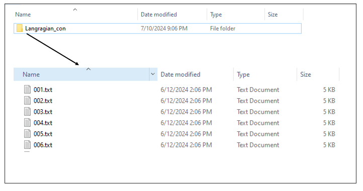
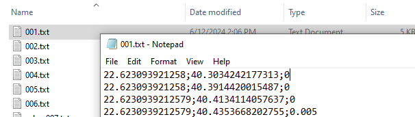
A typical Lagrangian output is a set of files representing the likelihood of a point moving from an origin (source) to a destination (target). This can be represented using a list of .txt/.csv files (as many as the origin points) including information for the destination probability. The .txt/.csv files need to be named in an increasing order. The name of the files need to correspond to the numbering of the points, in order for the algorithm to match the coordinates with the points.

Value

an edge list data.frame object, with the following columns:

• feature: feature name.

• from.X: longitude of the origin (source).

• from.Y: latitude of the origin (source).

• to.X: longitude of the destination (target).

• to.Y: latitude of the destination (target).

• weight: connection weight.

See Also

preprocess_graphs, get_metrics

Examples

# Read connectivity files from folder and combine them
combined_edge_list <- preprocess_graphs(system.file("external",
                                        package="priorCON"),
                                        header = FALSE, sep =";")
head(combined_edge_list)

##  feature   from.X   from.Y     to.X     to.Y weight
## 1     f1 22.62309 40.30342 22.62309 40.30342  0.000
## 2     f1 22.62309 40.30342 22.62309 40.39144  0.000
## 3     f1 22.62309 40.30342 22.62309 40.41341  0.000
## 4     f1 22.62309 40.30342 22.62309 40.43537  0.005
## 5     f1 22.62309 40.30342 22.62309 40.45731  0.000
## 6     f1 22.62309 40.30342 22.65266 40.30342  0.000