Help for package powerly

Title:

Sample Size Analysis for Psychological Networks and More

Version:

1.8.6

Description:

An implementation of the sample size computation method for network models proposed by Constantin et al. (2021) <doi:10.31234/osf.io/j5v7u>. The implementation takes the form of a three-step recursive algorithm designed to find an optimal sample size given a model specification and a performance measure of interest. It starts with a Monte Carlo simulation step for computing the performance measure and a statistic at various sample sizes selected from an initial sample size range. It continues with a monotone curve-fitting step for interpolating the statistic across the entire sample size range. The final step employs stratified bootstrapping to quantify the uncertainty around the fitted curve.

License:

MIT + file LICENSE

URL:

https://powerly.dev

BugReports:

https://github.com/mihaiconstantin/powerly/issues

Imports:

R6, progress, parallel, splines2, quadprog, osqp, bootnet, qgraph, ggplot2, rlang, mvtnorm, patchwork

Encoding:

UTF-8

RoxygenNote:

7.2.1

Collate:

'Backend.R' 'Basis.R' 'Model.R' 'GgmModel.R' 'Interpolation.R' 'Spline.R' 'StepThree.R' 'StepTwo.R' 'Statistic.R' 'PowerStatistic.R' 'StatisticFactory.R' 'ModelFactory.R' 'StepOne.R' 'Range.R' 'Method.R' 'OsqpSolver.R' 'QuadprogSolver.R' 'Solver.R' 'SolverFactory.R' 'Validation.R' 'constants.R' 'exports.R' 'helpers.R' 'logo.R' 'powerly-package.R'

Suggests:

testthat (≥ 3.0.0)

Config/testthat/edition:

NeedsCompilation:

Packaged:

2022-09-09 13:41:09 UTC; mihai

Author:

Mihai Constantin

[aut, cre]

Maintainer:

Mihai Constantin <mihai@mihaiconstantin.com>

Repository:

CRAN

Date/Publication:

2022-09-09 14:10:01 UTC

Sample Size Analysis for Psychological Networks and More

Description

powerly is a package that implements the method by Constantin et al. (2021) for conducting sample size analysis for network models.

Details

The method implemented is implemented in the main function powerly(). The implementation takes the form of a three-step recursive algorithm designed to find an optimal sample size value given a model specification and an outcome measure of interest. It starts with a Monte Carlo simulation step for computing the outcome at various sample sizes. It continues with a monotone curve-fitting step for interpolating the outcome. The final step employs stratified bootstrapping to quantify the uncertainty around the fitted curve.

Author(s)

Maintainer: Mihai Constantin mihai@mihaiconstantin.com (ORCID)

The `powerly` package logo

Description

The logo is generated by make_logo() and displayed at package load time.

Usage

LOGO

Format

An object of class character of length 1.

Generate true model parameters

Description

Generate matrices of true model parameters for the supported true models. These matrices are intended to passed to the model_matrix argument of powerly().

Usage

generate_model(type, ...)

Arguments

type

Character string representing the type of true model. Possible values are "ggm" (the default).

...

Required arguments used for the generation of the true model. See the True Models section of powerly() for the arguments required for each true model.

Value

A matrix containing the model parameters.

Update package logo

Description

This function is meant for generating or updating the logo. After running this procedure we end up with what is stored in the LOGO constant.

Usage

make_logo(
  ascii_logo_path = "./inst/assets/logo/logo.txt",
  version = c(1, 0, 0)
)

Arguments

ascii_logo_path

A character string representing the path to the logo template.

version

A numerical vector of three positive integers representing the version of the package to append to the logo.

Value

The ASCII logo.

Plot the results of a sample size analysis

Description

This function plots the results for each step of the method.

Usage

## S3 method for class 'Method'
plot(
  x,
  step = 3,
  last = TRUE,
  save = FALSE,
  path = NULL,
  width = 14,
  height = 10,
  ...
)

Arguments

x

An object instance of class Method.

step

A single positive integer representing the method step that should be plotted. Possibles values are 1 for the first step, 2 for the second step, and 3 for the third step of the method.

last

A logical value indicating whether the last iteration of the method should be plotted. The default is TRUE, indicating that the last iteration should be plotted.

save

A logical value indicating whether the plot should be saved to a file on disk.

path

A character string representing the path (i.e., including the filename and extension) where the plot should be saved on disk. If NULL, the plot will be saved in the current working directory with a filename generated based on the current system time and a .pdf extension. See ggplot2::ggsave() for supported file types.

width

A single numerical value representing the desired plot width. The default unit is inches (i.e., set by ggplot2::ggsave()), unless overridden by providing the units argument via ....

height

A single numerical value representing the desired plot height. The default unit is inches (i.e., set by ggplot2::ggsave()), unless overridden by providing the units argument via ....

...

Optional arguments to be passed to ggplot2::ggsave().

Value

An ggplot2::ggplot object containing the plot for the requested step of the method. The plot object returned can be further modified and also contains the patchwork class applied.

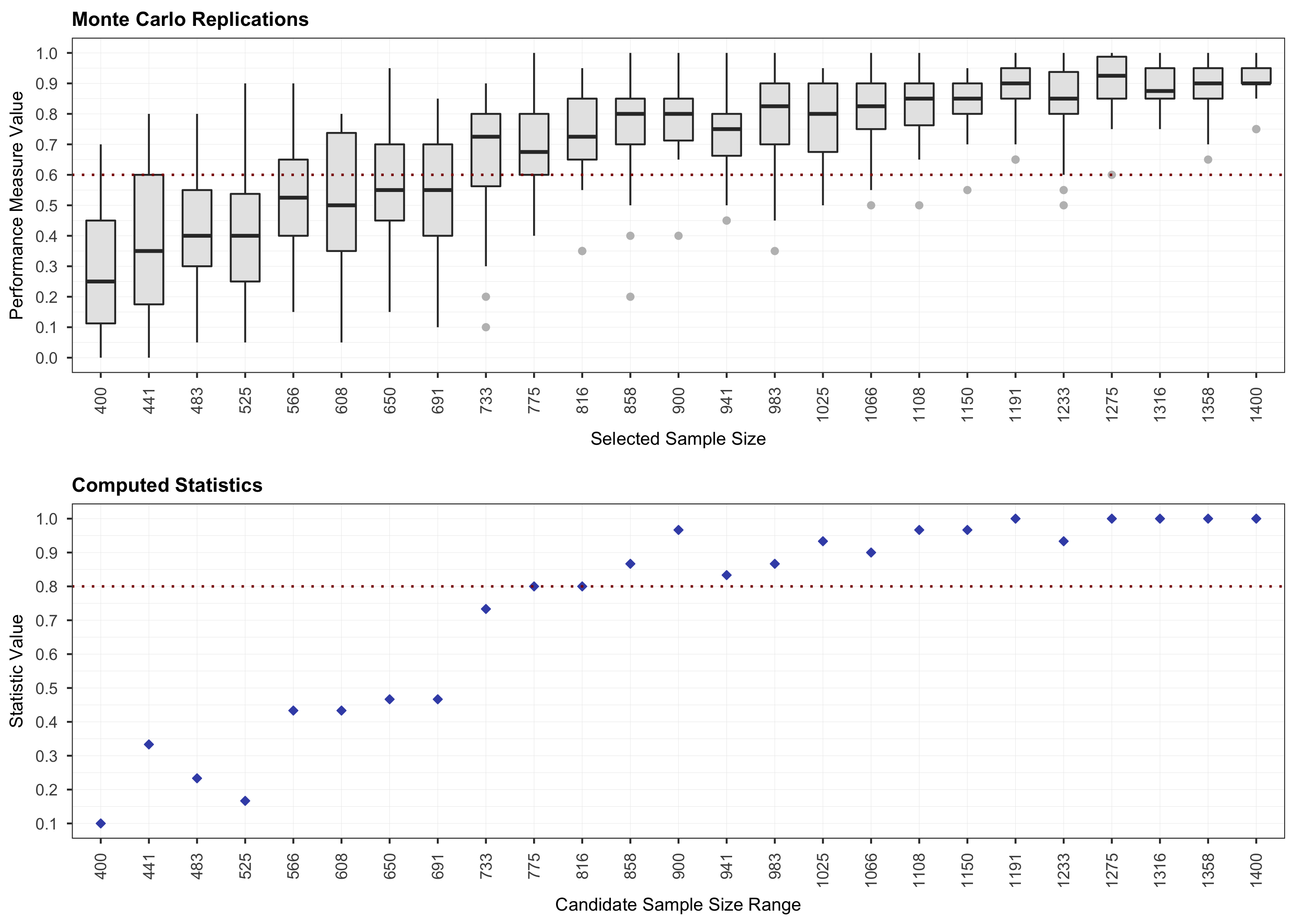
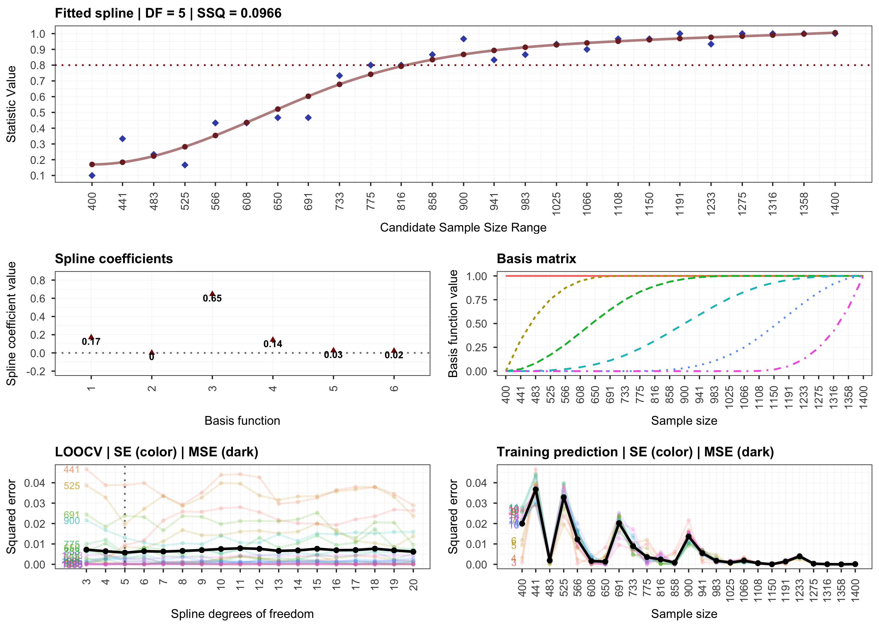
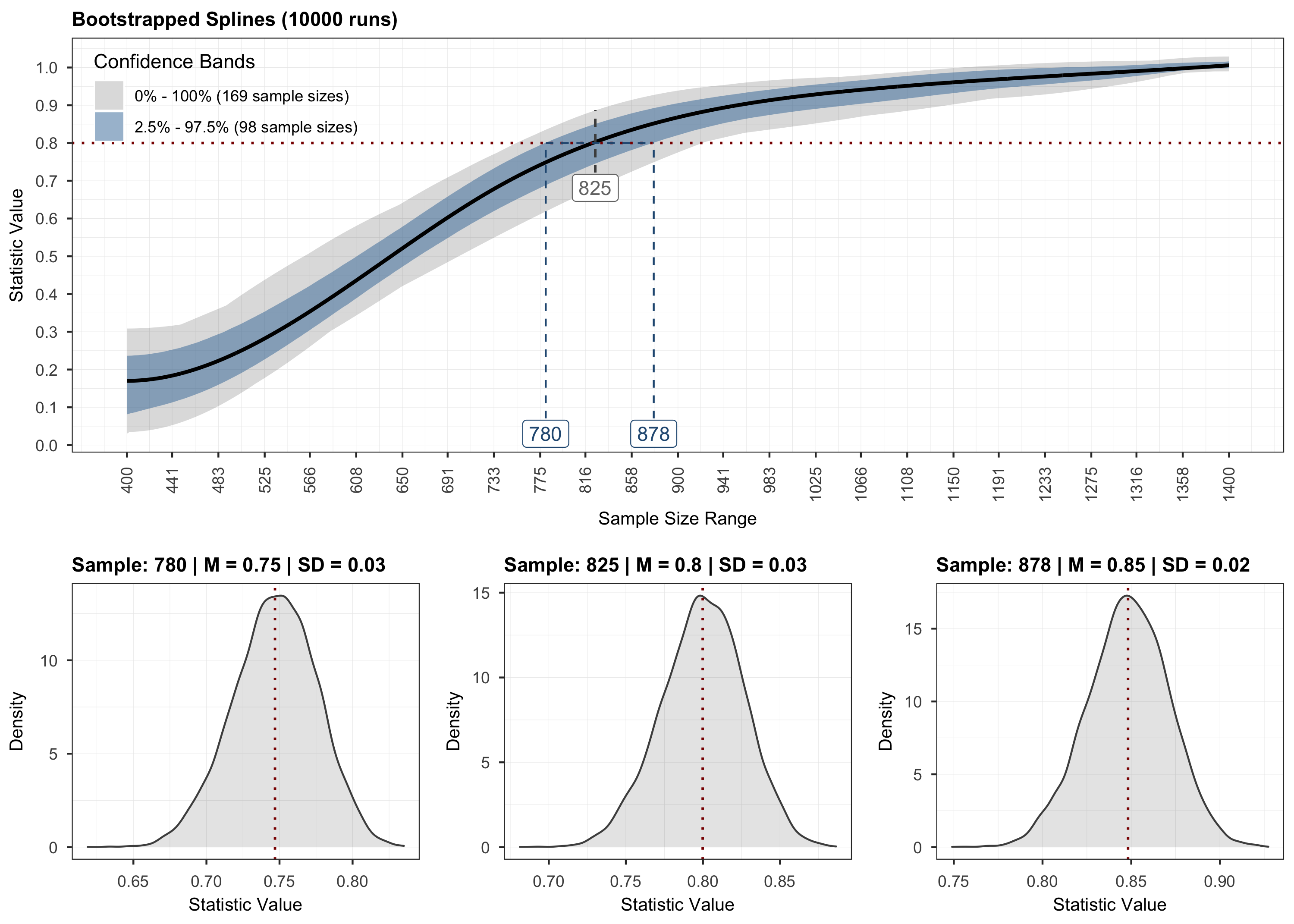
Example of a plot for each step of the method: Step 1: Monte Carlo Replications Example Step 1 Step 2: Curve Fitting Example Step 2 Step 3: Bootstrapping Example Step 3

Plot `StepOne` objects

Description

This function plots the results for Step 1 of the method.

Usage

## S3 method for class 'StepOne'
plot(x, save = FALSE, path = NULL, width = 14, height = 10, ...)

Arguments

x

An object instance of class StepOne.

save

A logical value indicating whether the plot should be saved to a file on disk.

path

width

A single numerical value representing the desired plot width. The default unit is inches (i.e., set by ggplot2::ggsave()), unless overridden by providing the units argument via ....

height

A single numerical value representing the desired plot height. The default unit is inches (i.e., set by ggplot2::ggsave()), unless overridden by providing the units argument via ....

...

Optional arguments to be passed to ggplot2::ggsave().

Value

An ggplot2::ggplot object containing the plot for a StepOne object that can be further modified. The object returned also contains the patchwork class applied.

Example of a plot: Example Step 1

Plot `StepThree` objects

Description

This function plots the results for Step 3 of the method.

Usage

## S3 method for class 'StepThree'
plot(x, save = FALSE, path = NULL, width = 14, height = 10, ...)

Arguments

x

An object instance of class StepThree.

save

A logical value indicating whether the plot should be saved to a file on disk.

path

width

A single numerical value representing the desired plot width. The default unit is inches (i.e., set by ggplot2::ggsave()), unless overridden by providing the units argument via ....

height

A single numerical value representing the desired plot height. The default unit is inches (i.e., set by ggplot2::ggsave()), unless overridden by providing the units argument via ....

...

Optional arguments to be passed to ggplot2::ggsave().

Value

An ggplot2::ggplot object containing the plot for a StepThree object that can be further modified. The object returned also contains the patchwork class applied.

Example of a plot: Example Step 3

Plot `StepTwo` objects

Description

This function plots the results for Step 2 of the method.

Usage

## S3 method for class 'StepTwo'
plot(x, save = FALSE, path = NULL, width = 14, height = 10, ...)

Arguments

x

An object instance of class StepTwo.

save

A logical value indicating whether the plot should be saved to a file on disk.

path

width

A single numerical value representing the desired plot width. The default unit is inches (i.e., set by ggplot2::ggsave()), unless overridden by providing the units argument via ....

height

A single numerical value representing the desired plot height. The default unit is inches (i.e., set by ggplot2::ggsave()), unless overridden by providing the units argument via ....

...

Optional arguments to be passed to ggplot2::ggsave().

Value

An ggplot2::ggplot object containing the plot for a StepTwo object that can be further modified. The object returned also contains the patchwork class applied.

Example of a plot: Example Step 2

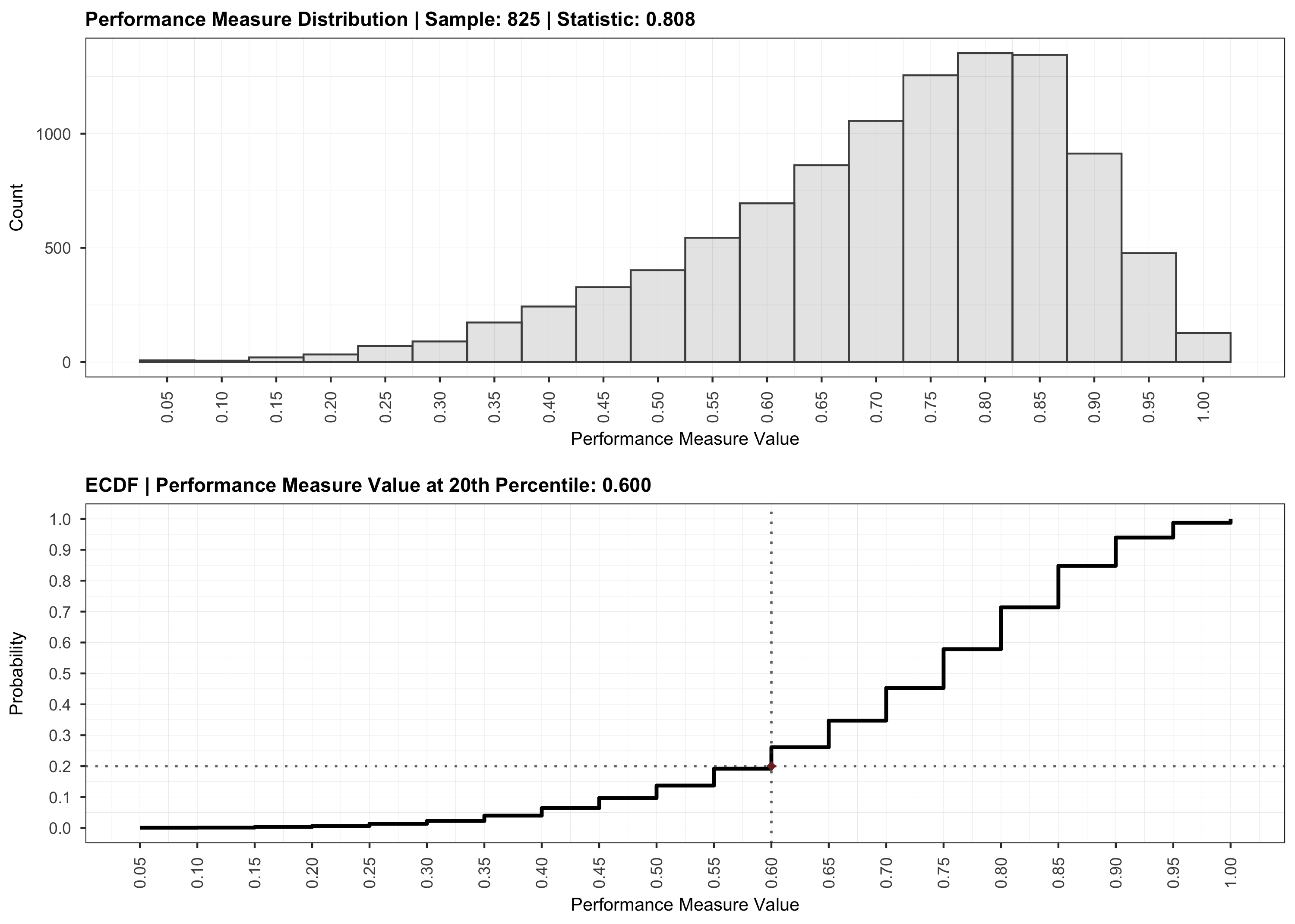
Plot the results of a sample size analysis validation

Description

This function plots the results for of a sample size analysis validation.

Usage

## S3 method for class 'Validation'
plot(x, save = FALSE, path = NULL, width = 14, height = 10, bins = 20, ...)

Arguments

x

An object instance of class Validation.

save

A logical value indicating whether the plot should be saved to a file on disk.

path

width

A single numerical value representing the desired plot width. The default unit is inches (i.e., set by ggplot2::ggsave()), unless overridden by providing the units argument via ....

height

A single numerical value representing the desired plot height. The default unit is inches (i.e., set by ggplot2::ggsave()), unless overridden by providing the units argument via ....

bins

A single positive integer passed to ggplot2::geom_histogram() representing the number of bins to use for the histogram plot. The default value is 20.

...

Optional arguments to be passed to ggplot2::ggsave().

Value

An ggplot2::ggplot object containing the plot for the validation procedure. The plot object returned can be further modified and also contains the patchwork class applied.

Example of a validation plot: Example Validation

Fetch `ggplot2` theme settings.

Description

This function is used to create reusable ggplot2 theme settings.

Usage

plot_settings()

Value

A list of ggplot2 layers.

Perform sample size analysis

Description

Run an iterative three-step Monte Carlo method and return the sample sizes required to obtain a certain value for a performance measure of interest (e.g., sensitivity) given a hypothesized network structure.

Usage

powerly(
  range_lower,
  range_upper,
  samples = 30,
  replications = 30,
  model = "ggm",
  ...,
  model_matrix = NULL,
  measure = "sen",
  statistic = "power",
  measure_value = 0.6,
  statistic_value = 0.8,
  monotone = TRUE,
  increasing = TRUE,
  spline_df = NULL,
  solver_type = "quadprog",
  boots = 10000,
  lower_ci = 0.025,
  upper_ci = 0.975,
  tolerance = 50,
  iterations = 10,
  cores = NULL,
  backend_type = NULL,
  save_memory = FALSE,
  verbose = TRUE
)

Arguments

range_lower

A single positive integer representing the lower bound of the candidate sample size range.

range_upper

A single positive integer representing the upper bound of the candidate sample size range.

samples

A single positive integer representing the number of sample sizes to select from the candidate sample size range.

replications

A single positive integer representing the number of Monte Carlo replications to perform for each sample size selected from the candidate range.

model

A character string representing the type of true model to find a sample size for. Possible values are "ggm" (the default).

...

Required arguments used for the generation of the true model. See the True Models section for the arguments required for each true model.

model_matrix

A square matrix representing the true model. See the True Models section for what this matrix should look like depending on the true model selected.

measure

A character string representing the type of performance measure of interest. Possible values are "sen" (i.e., sensitivity; the default), "spe" (i.e., specificity), "mcc" (i.e., Matthews correlation), and "rho" (i.e., Pearson correlation). See the True Models section for the performance measures available for each type of true model supported.

statistic

A character string representing the type of statistic to be computed on the values obtained for the performance measures. Possible values are "power" (the default).

measure_value

A single numerical value representing the desired value for the performance measure of interest. The default is 0.6 (i.e., for the measure = "sen"). See the Performance Measures section for the range of values allowed for each performance measure.

statistic_value

A single numerical value representing the desired value for the statistic of interest. The default is 0.8 (i.e., for the statistic = "power"). See the "Statistics" section for the range of values allowed for each statistic.

monotone

A logical value indicating whether a monotonicity assumption should be placed on the values of the performance measure. The default is TRUE meaning that the performance measure changes as a function of sample size (i.e., either by increasing or decreasing as the sample size goes up). The alternative FALSE indicates that the performance measure it is not assumed to change as a function a sample size.

increasing

A logical value indicating whether the performance measure is assumed to follow a non-increasing or non-decreasing trend. TRUE (the default) indicates a non-decreasing trend (i.e., the performance measure increases as the sample size goes up). FALSE indicates a non-increasing trend (i.e., the performance measure decreases as the sample size goes up).

spline_df

A vector of positive integers representing the degrees of freedom considered for constructing the spline basis, or NULL. The best degree of freedom is selected based on Leave One Out Cross-Validation. If NULL (the default) is provided, a vector of degrees of freedom is automatically created with all integers between 3 and 20.

solver_type

A character string representing the type of the quadratic solver used for estimating the spline coefficients. Possible values are "quadprog" (the default) and "osqp". Currently, the "osqp" solver does not play nicely with R's parallel::parallel package and cannot be used when powerly is ran in parallel.

boots

A positive integer representing the number of bootstrap runs to perform on the matrix of performance measures in order to obtained bootstrapped values for the statistic of interest. The default is 10000.

lower_ci

A single numerical value indicating the lower bound for the confidence interval to be computed on the bootstrapped statistics. The default is 0.025 (i.e., 2.5%).

upper_ci

A single numerical value indicating the upper bound for the confidence to be computed on the bootstrapped statistics. The default is 0.975 (i.e., 97.5%).

tolerance

A single positive integer representing the width at the candidate sample size range at which the algorithm is considered to have converge. The default is 50, meaning that the algorithm will stop running when the difference between the upper and the lower bound of the candidate range shrinks to 50 sample sizes.

iterations

A single positive integer representing the number of iterations the algorithm is allowed to run. The default is 10.

cores

A single positive positive integer representing the number of cores to use for running the algorithm in parallel, or NULL. If NULL (the default) the algorithm will run sequentially.

backend_type

A character string indicating the type of cluster to create for running the algorithm in parallel, or NULL. Possible values are "psock" and "fork". If NULL the backend is determined based on the computer architecture (i.e., fork for Unix and MacOS and psock for Windows).

save_memory

A logical value indicating whether to save memory by only storing the results for the last iteration of the method. The default TRUE indicates that only the last iteration should be saved.

verbose

A logical value indicating whether information about the status of the algorithm should be printed while running. The default is TRUE.

Details

This function represents the implementation of the method introduced by Constantin et al. (2021; see doi:10.31234/osf.io/j5v7u) for performing a priori sample size analysis in the context of network models. The method takes the form of a three-step recursive algorithm designed to find an optimal sample size value given a model specification and an outcome measure of interest (e.g., sensitivity). It starts with a Monte Carlo simulation step for computing the outcome of interest at various sample sizes. It continues with a monotone non-decreasing curve-fitting step for interpolating the outcome. The final step employs a stratified bootstrapping scheme to account for the uncertainty around the recommendation provided. The method runs the three steps recursively until the candidate sample size range used for the search shrinks below a specified value.

Value

An R6::R6Class() instance of Method class that contains the results for each step of the method for the last and previous iterations.

Main fields:

⁠$duration⁠: The time in seconds elapsed during the method run.
⁠$iteration⁠: The number of iterations performed.
⁠$converged⁠: Whether the method converged.
⁠$previous⁠: The results during the previous iteration.
⁠$range⁠: The candidate sample size range.
⁠$step_1⁠: The results for Step 1.
⁠$step_2⁠: The results for Step 2.
⁠$step_3⁠: The results for Step 3.
⁠$recommendation⁠: The sample size recommendation(s).

The plot method can be called on the return value to visualize the results. See plot.Method() for more information on how to plot the method results.

for Step 1: plot(results, step = 1)
for Step 2: plot(results, step = 2)
for Step 3: plot(results, step = 3)

True Models

Gaussian Graphical Model (GGM)

type: cross-sectional
symbol: ggm
... arguments for generating true models:
- nodes: A single positive integer representing the number of nodes in the network (e.g., 10).
- density: A single numerical value indicating the density of the network (e.g., 0.4).
- positive: A single numerical value representing the proportion of positive edges in the network (e.g., 0.9 for 90% positive edges).
- range: A length two numerical value indicating the uniform interval from where to sample values for the partial correlations coefficients (e.g., c(0.5, 1)).
- constant: A single numerical value representing the constant described by Yin and Li (2011).
- for more information on the arguments see:
  - the function bootnet::genGGM()
  - Yin, J., and Li, H. (2011). A sparse conditional gaussian graphical model for analysis of genetical genomics data. The annals of applied statistics, 5(4), 2630.
supported performance measures: sen, spe, mcc, rho

Performance Measures

Performance Measure	Symbol	Lower	Upper
Sensitivity	`sen`	`0.00`	`1.00`
Specificity	`spe`	`0.00`	`1.00`
Matthews correlation	`mcc`	`-1.00`	`1.00`
Pearson correlation	`rho`	`-1.00`	`1.00`

Statistics

Statistics	Symbol	Lower	Upper
Power	`power`	`0.00`	`1.00`

Requests

If you would like to support a new model, performance measure, or statistic, please open a pull request on GitHub at github.com/mihaiconstantin/powerly/pulls.
To request a new model, performance measure, or statistic, please submit your request at github.com/mihaiconstantin/powerly/issues. If possible, please also include references discussing the topics you are requesting.
Alternatively, you can get in touch at ⁠mihai at mihaiconstantin dot com⁠.

References

Constantin, M. A., Schuurman, N. K., & Vermunt, J. (2021). A General Monte Carlo Method for Sample Size Analysis in the Context of Network Models. PsyArXiv. doi:10.31234/osf.io/j5v7u

Examples

# Suppose we want to find the sample size for observing a sensitivity of `0.6`
# with a probability of `0.8`, for a GGM true model consisting of `10` nodes
# with a density of `0.4`.

# We can run the method for an arbitrarily generated true model that matches
# those characteristics (i.e., number of nodes and density).
results <- powerly(
    range_lower = 300,
    range_upper = 1000,
    samples = 30,
    replications = 30,
    measure = "sen",
    statistic = "power",
    measure_value = .6,
    statistic_value = .8,
    model = "ggm",
    nodes = 10,
    density = .4,
    cores = 2,
    verbose = TRUE
)

# Or we omit the `nodes` and `density` arguments and specify directly the edge
# weights matrix via the `model_matrix` argument.

# To get a matrix of edge weights we can use the `generate_model()` function.
true_model <- generate_model(type = "ggm", nodes = 10, density = .4)

# Then, supply the true model to the algorithm directly.
results <- powerly(
    range_lower = 300,
    range_upper = 1000,
    samples = 30,
    replications = 30,
    measure = "sen",
    statistic = "power",
    measure_value = .6,
    statistic_value = .8,
    model = "ggm",
    model_matrix = true_model,
    cores = 2,
    verbose = TRUE
)

# To visualize the results, we can use the `plot` S3 method and indicating the
# step that should be plotted.
plot(results, step = 1)
plot(results, step = 2)
plot(results, step = 3)

# To see a summary of the results, we can use the `summary` S3 method.
summary(results)

Provide a summary of the sample size analysis results

Description

This function summarizes the objects of class Method and provides information about the method run and the sample size recommendation.

Usage

## S3 method for class 'Method'
summary(object, ...)

Arguments

object

An object instance of class Method.

...

Other optional arguments currently not in use.

Provide a summary of the sample size analysis validation results

Description

This function summarizes the objects of class Validation providing information about the validation procedure and results.

Usage

## S3 method for class 'Validation'
summary(object, ...)

Arguments

object

An object instance of class Validation.

...

Other optional arguments currently not in use.

Validate a sample size analysis

Description

This function can be used to validate the recommendation obtained from a sample size analysis.

Usage

validate(
  method,
  replications = 3000,
  cores = NULL,
  backend_type = NULL,
  verbose = TRUE
)

Arguments

method

An object of class Method produced by running powerly().

replications

A single positive integer representing the number of Monte Carlo simulations to perform for the recommended sample size. The default is 1000. Whenever possible, a value of 10000 should be preferred for a higher accuracy of the validation results.

cores

A single positive positive integer representing the number of cores to use for running the validation in parallel, or NULL. If NULL (the default) the validation will run sequentially.

backend_type

A character string indicating the type of cluster to create for running the validation in parallel, or NULL. Possible values are "psock" and "fork". If NULL the backend is determined based on the computer architecture (i.e., fork for Unix and MacOS and psock for Windows).

verbose

A logical value indicating whether information about the status of the validation should be printed while running. The default is TRUE.

Details

The sample sizes used during the validation procedure is automatically extracted from the method argument.

Value

An R6::R6Class() instance of Validation class that contains the results of the validation.

Main fields:

⁠$sample⁠: The sample size used for the validation.
⁠$measures⁠: The performance measures observed during validation.
⁠$statistic⁠: The statistic computed on the performance measures.
⁠$percentile_value⁠: The performance measure value at the desired percentile.
⁠$validator⁠: An R6::R6Class() instance of StepOne class.

The plot S3 method can be called on the return value to visualize the validation results (i.e., see plot.Validation()).

plot(validation)

Examples

# Perform a sample size analysis.
results <- powerly(
    range_lower = 300,
    range_upper = 1000,
    samples = 30,
    replications = 30,
    measure = "sen",
    statistic = "power",
    measure_value = .6,
    statistic_value = .8,
    model = "ggm",
    nodes = 10,
    density = .4,
    cores = 2,
    verbose = TRUE
)

# Validate the recommendation obtained during the analysis.
validation <- validate(results, cores = 2)

# Plot the validation results.
plot(validation)

# To see a summary of the validation procedure, we can use the `summary` S3 method.
summary(validation)

Sample Size Analysis for Psychological Networks and More

Description

Details

Author(s)

See Also

The powerly package logo

Description

Usage

Format

Generate true model parameters

Description

Usage

Arguments

Value

See Also

Update package logo

Description

Usage

Arguments

Value

Plot the results of a sample size analysis

Description

Usage

Arguments

Value

See Also

Plot StepOne objects

Description

Usage

Arguments

Value

See Also

Plot StepThree objects

Description

Usage

Arguments

Value

See Also

Plot StepTwo objects

Description

Usage

Arguments

Value

See Also

Plot the results of a sample size analysis validation

Description

Usage

Arguments

Value

See Also

Fetch ggplot2 theme settings.

Description

Usage

Value

Perform sample size analysis

Description

Usage

Arguments

Details

Value

True Models

Performance Measures

Statistics

Requests

References

See Also

Examples

Provide a summary of the sample size analysis results

Description

Usage

Arguments

See Also

Provide a summary of the sample size analysis validation results

Description

Usage

Arguments

See Also

Validate a sample size analysis

Description

Usage

The `powerly` package logo

Plot `StepOne` objects

Plot `StepThree` objects

Plot `StepTwo` objects

Fetch `ggplot2` theme settings.