Title:	Infrastructure for Partially Observable Markov Decision Processes (POMDP)
Version:	1.2.5
Date:	2025-05-29
Description:	Provides the infrastructure to define and analyze the solutions of Partially Observable Markov Decision Process (POMDP) models. Interfaces for various exact and approximate solution algorithms are available including value iteration, point-based value iteration and SARSOP. Hahsler and Cassandra <doi:10.32614/RJ-2024-021>.
Classification/ACM:	G.4, G.1.6, I.2.6
URL:	https://github.com/mhahsler/pomdp
BugReports:	https://github.com/mhahsler/pomdp/issues
Depends:	R (≥ 3.5.0)
Imports:	pomdpSolve (≥ 1.0.4), processx, stats, methods, Matrix, Rcpp, foreach, igraph
SystemRequirements:	C++17
LinkingTo:	Rcpp
Suggests:	knitr, rmarkdown, gifski, testthat, Ternary, visNetwork, sarsop, doParallel
VignetteBuilder:	knitr
Encoding:	UTF-8
License:	GPL (≥ 3)
Copyright:	Copyright (C) Michael Hahsler and Hossein Kamalzadeh.
RoxygenNote:	7.3.2
Collate:	'AAA_check_installed.R' 'AAA_pomdp-package.R' 'AAA_shorten.R' 'Cliff_walking.R' 'DynaMaze.R' 'POMDP.R' 'MDP.R' 'MDP_policy_functions.R' 'Maze.R' 'POMDP_file_examples.R' 'RcppExports.R' 'RussianTiger.R' 'Tiger.R' 'Windy_gridworld.R' 'accessors.R' 'accessors_reward.R' 'accessors_trans_obs.R' 'actions.R' 'add_policy.R' 'check_and_fix_MDP.R' 'colors.R' 'estimate_belief_for_nodes.R' 'foreach_helper.R' 'gridworld.R' 'make_partially_observable.R' 'optimal_action.R' 'plot_belief_space.R' 'plot_policy_graph.R' 'policy.R' 'policy_graph.R' 'print.text.R' 'projection.R' 'queue.R' 'reachable_and_absorbing.R' 'read_write_POMDP.R' 'read_write_pomdp_solve.R' 'regret.R' 'reward.R' 'round_stochchastic.R' 'sample_belief_space.R' 'simulate_MDP.R' 'simulate_POMDP.R' 'solve_MDP.R' 'solve_POMDP.R' 'solve_SARSOP.R' 'stack.R' 'transition_graph.R' 'update_belief.R' 'value_function.R' 'which_max_random.R'
NeedsCompilation:	yes
Packaged:	2025-05-29 19:51:57 UTC; mhahsler
Author:	Michael Hahsler [aut, cph, cre], Hossein Kamalzadeh [ctb]
Maintainer:	Michael Hahsler <mhahsler@lyle.smu.edu>
Repository:	CRAN
Date/Publication:	2025-05-29 20:40:02 UTC

pomdp: Infrastructure for Partially Observable Markov Decision Processes (POMDP)

Description

Provides the infrastructure to define and analyze the solutions of Partially Observable Markov Decision Process (POMDP) models. Interfaces for various exact and approximate solution algorithms are available including value iteration, point-based value iteration and SARSOP. Hahsler and Cassandra doi:10.32614/RJ-2024-021.

Key functions

• Problem specification: POMDP, MDP

• Solvers: solve_POMDP(), solve_MDP(), solve_SARSOP()

Author(s)

Maintainer: Michael Hahsler mhahsler@lyle.smu.edu (ORCID) [copyright holder]

Other contributors:

• Hossein Kamalzadeh [contributor]

See Also

Useful links:

• https://github.com/mhahsler/pomdp

• Report bugs at https://github.com/mhahsler/pomdp/issues

Cliff Walking Gridworld MDP

Description

The cliff walking gridworld MDP example from Chapter 6 of the textbook "Reinforcement Learning: An Introduction."

Format

An object of class MDP.

Details

The cliff walking gridworld has the following layout:

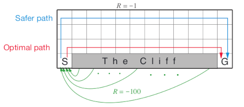
The gridworld is represented as a 4 x 12 matrix of states. The states are labeled with their x and y coordinates. The start state is in the bottom left corner. Each action has a reward of -1, falling off the cliff has a reward of -100 and returns the agent back to the start. The episode is finished once the agent reaches the absorbing goal state in the bottom right corner. No discounting is used (i.e., \gamma = 1).

References

Richard S. Sutton and Andrew G. Barto (2018). Reinforcement Learning: An Introduction Second Edition, MIT Press, Cambridge, MA.

See Also

Other MDP_examples: DynaMaze, MDP(), Maze, Windy_gridworld

Other gridworld: DynaMaze, Maze, Windy_gridworld, gridworld

Examples

data(Cliff_walking)
Cliff_walking

gridworld_matrix(Cliff_walking)
gridworld_matrix(Cliff_walking, what = "labels")

# The Goal is an absorbing state 
which(absorbing_states(Cliff_walking))

# visualize the transition graph
gridworld_plot_transition_graph(Cliff_walking)

# solve using different methods
sol <- solve_MDP(Cliff_walking) 
sol
policy(sol)
gridworld_plot_policy(sol)

sol <- solve_MDP(Cliff_walking, method = "q_learning", N = 100) 
sol
policy(sol)
gridworld_plot_policy(sol)

sol <- solve_MDP(Cliff_walking, method = "sarsa", N = 100) 
sol
policy(sol)
gridworld_plot_policy(sol)

sol <- solve_MDP(Cliff_walking, method = "expected_sarsa", N = 100, alpha = 1) 
policy(sol)
gridworld_plot_policy(sol)

The Dyna Maze

Description

The Dyna Maze from Chapter 8 of the textbook "Reinforcement Learning: An Introduction."

Format

An object of class MDP.

Details

The simple 6x9 maze with a few walls.

References

Richard S. Sutton and Andrew G. Barto (2018). Reinforcement Learning: An Introduction Second Edition, MIT Press, Cambridge, MA.

See Also

Other MDP_examples: Cliff_walking, MDP(), Maze, Windy_gridworld

Other gridworld: Cliff_walking, Maze, Windy_gridworld, gridworld

Other MDP_examples: Cliff_walking, MDP(), Maze, Windy_gridworld

Other gridworld: Cliff_walking, Maze, Windy_gridworld, gridworld

Examples

data(DynaMaze)

DynaMaze

gridworld_matrix(DynaMaze)
gridworld_matrix(DynaMaze, what = "labels")

gridworld_plot_transition_graph(DynaMaze)

Define an MDP Problem

Description

Defines all the elements of a finite state-space MDP problem.

Usage

MDP(
  states,
  actions,
  transition_prob,
  reward,
  discount = 0.9,
  horizon = Inf,
  start = "uniform",
  info = NULL,
  name = NA
)

is_solved_MDP(x, stop = FALSE)

Arguments

Details

Markov decision processes (MDPs) are discrete-time stochastic control process with completely observable states. We implement here MDPs with a finite state space. similar to POMDP models, but without the observation model. The 'observations' column in the the reward specification is always missing.

make_partially_observable() reformulates an MDP as a POMDP by adding an observation model with one observation per state that reveals the current state. This is achieved by adding identity observation probability matrices.

More details on specifying the model components can be found in the documentation for POMDP.

Value

The function returns an object of class MDP which is list with the model specification. solve_MDP() reads the object and adds a list element called 'solution'.

Author(s)

Michael Hahsler

See Also

Other MDP: MDP2POMDP, MDP_policy_functions, accessors, actions(), add_policy(), gridworld, reachable_and_absorbing, regret(), simulate_MDP(), solve_MDP(), transition_graph(), value_function()

Other MDP_examples: Cliff_walking, DynaMaze, Maze, Windy_gridworld

Examples

# Michael's Sleepy Tiger Problem is like the POMDP Tiger problem, but
# has completely observable states because the tiger is sleeping in front
# of the door. This makes the problem an MDP.

STiger <- MDP(
  name = "Michael's Sleepy Tiger Problem",
  discount = .9,

  states = c("tiger-left" , "tiger-right"),
  actions = c("open-left", "open-right", "do-nothing"),
  start = "uniform",

  # opening a door resets the problem
  transition_prob = list(
    "open-left" =  "uniform",
    "open-right" = "uniform",
    "do-nothing" = "identity"),

  # the reward helper R_() expects: action, start.state, end.state, observation, value
  reward = rbind(
    R_("open-left",  "tiger-left",  v = -100),
    R_("open-left",  "tiger-right", v =   10),
    R_("open-right", "tiger-left",  v =   10),
    R_("open-right", "tiger-right", v = -100),
    R_("do-nothing",                v =    0)
  )
)

STiger

sol <- solve_MDP(STiger)
sol

policy(sol)
plot_value_function(sol)

# convert the MDP into a POMDP and solve
STiger_POMDP <- make_partially_observable(STiger)
sol2 <- solve_POMDP(STiger_POMDP)
sol2

policy(sol2)
plot_value_function(sol2, ylim = c(80, 120))

Convert between MDPs and POMDPs

Description

Convert a MDP into POMDP by adding an observation model or a POMDP into a MDP by making the states observable.

Usage

make_partially_observable(x, observations = NULL, observation_prob = NULL)

make_fully_observable(x)

Arguments

Details

make_partially_observable() adds an observation model to an MDP. If no observations and observation probabilities are provided, then an observation for each state is created with identity observation matrices. This means we have a fully observable model encoded as a POMDP.

make_fully_observable() removes the observation model from a POMDP and returns an MDP.

Value

a MDP or a POMDP object.

Author(s)

Michael Hahsler

See Also

Other MDP: MDP(), MDP_policy_functions, accessors, actions(), add_policy(), gridworld, reachable_and_absorbing, regret(), simulate_MDP(), solve_MDP(), transition_graph(), value_function()

Other POMDP: POMDP(), accessors, actions(), add_policy(), plot_belief_space(), projection(), reachable_and_absorbing, regret(), sample_belief_space(), simulate_POMDP(), solve_POMDP(), solve_SARSOP(), transition_graph(), update_belief(), value_function(), write_POMDP()

Examples

# Turn the Maze MDP into a partially observable problem.
# Here each state has an observation, so it is still a fully observable problem
# encoded as a POMDP.
data("Maze")
Maze

Maze_POMDP <- make_partially_observable(Maze)
Maze_POMDP

sol <- solve_POMDP(Maze_POMDP)
policy(sol)
simulate_POMDP(sol, n = 1, horizon = 100, return_trajectories = TRUE)$trajectories

# Make the Tiger POMDP fully observable
data("Tiger")
Tiger

Tiger_MDP <- make_fully_observable(Tiger)
Tiger_MDP

sol <- solve_MDP(Tiger_MDP)
policy(sol)
# The result is not exciting since we can observe where the tiger is!

Functions for MDP Policies

Description

Implementation several functions useful to deal with MDP policies.

Usage

q_values_MDP(model, U = NULL)

MDP_policy_evaluation(
  pi,
  model,
  U = NULL,
  k_backups = 1000,
  theta = 0.001,
  verbose = FALSE
)

greedy_MDP_action(s, Q, epsilon = 0, prob = FALSE)

random_MDP_policy(model, prob = NULL)

manual_MDP_policy(model, actions)

greedy_MDP_policy(Q)

Arguments

Details

Implemented functions are:

• q_values_MDP() calculates (approximates) Q-values for a given model using the Bellman optimality equation:

  q(s,a) = \sum_{s'} T(s'|s,a) [R(s,a) + \gamma U(s')]

  Q-values can be used as the input for several other functions.

• MDP_policy_evaluation() evaluates a policy \pi for a model and returns (approximate) state values by applying the Bellman equation as an update rule for each state and iteration k:

  U_{k+1}(s) =\sum_a \pi{a|s} \sum_{s'} T(s' | s,a) [R(s,a) + \gamma U_k(s')]

  In each iteration, all states are updated. Updating is stopped after k_backups iterations or after the largest update ||U_{k+1} - U_k||_\infty < \theta.

• greedy_MDP_action() returns the action with the largest Q-value given a state.

• random_MDP_policy(), manual_MDP_policy(), and greedy_MDP_policy() generates different policies. These policies can be added to a problem using add_policy().

Value

q_values_MDP() returns a state by action matrix specifying the Q-function, i.e., the action value for executing each action in each state. The Q-values are calculated from the value function (U) and the transition model.

MDP_policy_evaluation() returns a vector with (approximate) state values (U).

greedy_MDP_action() returns the action with the highest q-value for state s. If prob = TRUE, then a vector with the probability for each action is returned.

random_MDP_policy() returns a data.frame with the columns state and action to define a policy.

manual_MDP_policy() returns a data.frame with the columns state and action to define a policy.

greedy_MDP_policy() returns the greedy policy given Q.

Author(s)

Michael Hahsler

References

Sutton, R. S., Barto, A. G. (2020). Reinforcement Learning: An Introduction. Second edition. The MIT Press.

See Also

Other MDP: MDP(), MDP2POMDP, accessors, actions(), add_policy(), gridworld, reachable_and_absorbing, regret(), simulate_MDP(), solve_MDP(), transition_graph(), value_function()

Examples

data(Maze)
Maze

# create several policies:
# 1. optimal policy using value iteration
maze_solved <- solve_MDP(Maze, method = "value_iteration")
maze_solved
pi_opt <- policy(maze_solved)
pi_opt
gridworld_plot_policy(add_policy(Maze, pi_opt), main = "Optimal Policy")

# 2. a manual policy (go up and in some squares to the right)
acts <- rep("up", times = length(Maze$states))
names(acts) <- Maze$states
acts[c("s(1,1)", "s(1,2)", "s(1,3)")] <- "right"
pi_manual <- manual_MDP_policy(Maze, acts)
pi_manual
gridworld_plot_policy(add_policy(Maze, pi_manual), main = "Manual Policy")

# 3. a random policy
set.seed(1234)
pi_random <- random_MDP_policy(Maze)
pi_random
gridworld_plot_policy(add_policy(Maze, pi_random), main = "Random Policy")

# 4. an improved policy based on one policy evaluation and
#   policy improvement step.
u <- MDP_policy_evaluation(pi_random, Maze)
q <- q_values_MDP(Maze, U = u)
pi_greedy <- greedy_MDP_policy(q)
pi_greedy
gridworld_plot_policy(add_policy(Maze, pi_greedy), main = "Greedy Policy")

#' compare the approx. value functions for the policies (we restrict
#'    the number of backups for the random policy since it may not converge)
rbind(
  random = MDP_policy_evaluation(pi_random, Maze, k_backups = 100),
  manual = MDP_policy_evaluation(pi_manual, Maze),
  greedy = MDP_policy_evaluation(pi_greedy, Maze),
  optimal = MDP_policy_evaluation(pi_opt, Maze)
)

# For many functions, we first add the policy to the problem description
#   to create a "solved" MDP
maze_random <- add_policy(Maze, pi_random)
maze_random

# plotting
plot_value_function(maze_random)
gridworld_plot_policy(maze_random)

# compare to a benchmark
regret(maze_random, benchmark = maze_solved)

# calculate greedy actions for state 1
q <- q_values_MDP(maze_random)
q
greedy_MDP_action(1, q, epsilon = 0, prob = FALSE)
greedy_MDP_action(1, q, epsilon = 0, prob = TRUE)
greedy_MDP_action(1, q, epsilon = .1, prob = TRUE)

Steward Russell's 4x3 Maze Gridworld MDP

Description

The 4x3 maze is described in Chapter 17 of the textbook "Artificial Intelligence: A Modern Approach" (AIMA).

Format

An object of class MDP.

Details

The simple maze has the following layout:

    1234           Transition model:
   ######             .8 (action direction)
  1#   +#              ^
  2# # -#              |
  3#S   #         .1 <-|-> .1
   ######

We represent the maze states as a gridworld matrix with 3 rows and 4 columns. The states are labeled s(row, col) representing the position in the matrix. The # (state s(2,2)) in the middle of the maze is an obstruction and not reachable. Rewards are associated with transitions. The default reward (penalty) is -0.04. The start state marked with S is s(3,1). Transitioning to + (state s(1,4)) gives a reward of +1.0, transitioning to - (state s_(2,4)) has a reward of -1.0. Both these states are absorbing (i.e., terminal) states.

Actions are movements (up, right, down, left). The actions are unreliable with a .8 chance to move in the correct direction and a 0.1 chance to instead to move in a perpendicular direction leading to a stochastic transition model.

Note that the problem has reachable terminal states which leads to a proper policy (that is guaranteed to reach a terminal state). This means that the solution also converges without discounting (discount = 1).

References

Russell,9 S. J. and Norvig, P. (2020). Artificial Intelligence: A modern approach. 4rd ed.

See Also

Other MDP_examples: Cliff_walking, DynaMaze, MDP(), Windy_gridworld

Other gridworld: Cliff_walking, DynaMaze, Windy_gridworld, gridworld

Examples

# The problem can be loaded using data(Maze).

# Here is the complete problem definition:
gw <- gridworld_init(dim = c(3, 4), unreachable_states = c("s(2,2)"))
gridworld_matrix(gw)

# the transition function is stochastic so we cannot use the standard
# gridworld gw$transition_prob() function
T <- function(action, start.state, end.state) {
  action <- match.arg(action, choices = gw$actions)
  
  # absorbing states
  if (start.state %in% c('s(1,4)', 's(2,4)')) {
    if (start.state == end.state) return(1)
    else return(0)
  }
  
  # actions are stochastic so we cannot use gw$trans_prob
  if(action %in% c("up", "down")) error_direction <- c("right", "left")
  else error_direction <- c("up", "down")
  
  rc <- gridworld_s2rc(start.state)
  delta <- list(up = c(-1, 0), 
                down = c(+1, 0),
                right = c(0, +1), 
                left = c(0, -1))
  P <- matrix(0, nrow = 3, ncol = 4)

  add_prob <- function(P, rc, a, value) {
    new_rc <- rc + delta[[a]]
    if (!(gridworld_rc2s(new_rc) %in% gw$states))
      new_rc <- rc
    P[new_rc[1], new_rc[2]] <- P[new_rc[1], new_rc[2]] + value
    P
  }

  P <- add_prob(P, rc, action, .8)
  P <- add_prob(P, rc, error_direction[1], .1)
  P <- add_prob(P, rc, error_direction[2], .1)
  P[rbind(gridworld_s2rc(end.state))]
}

T("up", "s(3,1)", "s(2,1)")

R <- rbind(
 R_(end.state   = NA,     value = -0.04),
 R_(end.state   = 's(2,4)',  value = -1),
 R_(end.state   = 's(1,4)',  value = +1),
 R_(start.state = 's(2,4)',  value = 0),
 R_(start.state = 's(1,4)',  value = 0)
)


Maze <- MDP(
 name = "Stuart Russell's 3x4 Maze",
 discount = 1,
 horizon = Inf,
 states = gw$states,
 actions = gw$actions,
 start = "s(3,1)",
 transition_prob = T,
 reward = R,
 info = list(gridworld_dim = c(3, 4),
             gridworld_labels = list(
                "s(3,1)" = "Start",
                "s(2,4)" = "-1",
                "s(1,4)" = "Goal: +1"
                )
             )
)

Maze

str(Maze)

gridworld_matrix(Maze)
gridworld_matrix(Maze, what = "labels")

# find absorbing (terminal) states
which(absorbing_states(Maze))

maze_solved <- solve_MDP(Maze)
policy(maze_solved)

gridworld_matrix(maze_solved, what = "values")
gridworld_matrix(maze_solved, what = "actions")

gridworld_plot_policy(maze_solved)

Define a POMDP Problem

Description

Defines all the elements of a POMDP problem including the discount rate, the set of states, the set of actions, the set of observations, the transition probabilities, the observation probabilities, and rewards.

Usage

POMDP(
  states,
  actions,
  observations,
  transition_prob,
  observation_prob,
  reward,
  discount = 0.9,
  horizon = Inf,
  terminal_values = NULL,
  start = "uniform",
  info = NULL,
  name = NA
)

is_solved_POMDP(x, stop = FALSE, message = "")

is_timedependent_POMDP(x)

epoch_to_episode(x, epoch)

is_converged_POMDP(x, stop = FALSE, message = "")

O_(action = NA, end.state = NA, observation = NA, probability)

T_(action = NA, start.state = NA, end.state = NA, probability)

R_(action = NA, start.state = NA, end.state = NA, observation = NA, value)

Arguments

Details

In the following we use the following notation. The POMDP is a 7-duple:

(S,A,T,R, \Omega ,O, \gamma).

S is the set of states; A is the set of actions; T are the conditional transition probabilities between states; R is the reward function; \Omega is the set of observations; O are the conditional observation probabilities; and \gamma is the discount factor. We will use lower case letters to represent a member of a set, e.g., s is a specific state. To refer to the size of a set we will use cardinality, e.g., the number of actions is |A|.

Note that the observation model is in the literature often also denoted by the letter Z.

Names used for mathematical symbols in code

• S, s, s': ⁠'states', start.state', 'end.state'⁠

• A, a: ⁠'actions', 'action'⁠

• \Omega, o: ⁠'observations', 'observation'⁠

State names, actions and observations can be specified as strings or index numbers (e.g., start.state can be specified as the index of the state in states). For the specification as data.frames below, NA can be used to mean any start.state, end.state, action or observation. Note that some POMDP solvers and the POMDP file format use '*' for this purpose.

The specification below map to the format used by pomdp-solve (see http://www.pomdp.org).

Specification of transition probabilities: T(s' | s, a)

Transition probability to transition to state s' from given state s and action a. The transition probabilities can be specified in the following ways:

• A data.frame with columns exactly like the arguments of T_(). You can use rbind() with helper function T_() to create this data frame. Probabilities can be specified multiple times and the definition that appears last in the data.frame will take affect.

• A named list of matrices, one for each action. Each matrix is square with rows representing start states s and columns representing end states s'. Instead of a matrix, also the strings 'identity' or 'uniform' can be specified.

• A function with the same arguments are T_(), but no default values that returns the transition probability.

Specification of observation probabilities: O(o | a, s')

The POMDP specifies the probability for each observation o given an action a and that the system transitioned to the end state s'. These probabilities can be specified in the following ways:

• A data frame with columns named exactly like the arguments of O_(). You can use rbind() with helper function O_() to create this data frame. Probabilities can be specified multiple times and the definition that appears last in the data.frame will take affect.

• A named list of matrices, one for each action. Each matrix has rows representing end states s' and columns representing an observation o. Instead of a matrix, also the string 'uniform' can be specified.

• A function with the same arguments are O_(), but no default values that returns the observation probability.

Specification of the reward function: R(a, s, s', o)

The reward function can be specified in the following ways:

• A data frame with columns named exactly like the arguments of R_(). You can use rbind() with helper function R_() to create this data frame. Rewards can be specified multiple times and the definition that appears last in the data.frame will take affect.

• A list of lists. The list levels are 'action' and 'start.state'. The list elements are matrices with rows representing end states s' and columns representing an observation o.

• A function with the same arguments are R_(), but no default values that returns the reward.

To avoid overflow problems with rewards, reward values should stay well within the range of ⁠[-1e10, +1e10]⁠. -Inf can be used as the reward for unavailable actions and will be translated into a large negative reward for solvers that only support finite reward values.

Start Belief

The initial belief state of the agent is a distribution over the states. It is used to calculate the total expected cumulative reward printed with the solved model. The function reward() can be used to calculate rewards for any belief.

Some methods use this belief to decide which belief states to explore (e.g., the finite grid method).

Options to specify the start belief state are:

• A probability distribution over the states. That is, a vector of |S| probabilities, that add up to 1.

• The string "uniform" for a uniform distribution over all states.

• An integer in the range 1 to n to specify the index of a single starting state.

• A string specifying the name of a single starting state.

The default initial belief is a uniform distribution over all states.

Convergence

A infinite-horizon POMDP needs to converge to provide a valid value function and policy.

A finite-horizon POMDP may also converging to a infinite horizon solution if the horizon is long enough.

Time-dependent POMDPs

Time dependence of transition probabilities, observation probabilities and reward structure can be modeled by considering a set of episodes representing epoch with the same settings. The length of each episode is specified as a vector for horizon, where the length is the number of episodes and each value is the length of the episode in epochs. Transition probabilities, observation probabilities and/or reward structure can contain a list with the values for each episode. The helper function epoch_to_episode() converts an epoch to the episode it belongs to.

Value

The function returns an object of class POMDP which is list of the model specification. solve_POMDP() reads the object and adds a list element named 'solution'.

Author(s)

Hossein Kamalzadeh, Michael Hahsler

References

pomdp-solve website: http://www.pomdp.org

See Also

Other POMDP: MDP2POMDP, accessors, actions(), add_policy(), plot_belief_space(), projection(), reachable_and_absorbing, regret(), sample_belief_space(), simulate_POMDP(), solve_POMDP(), solve_SARSOP(), transition_graph(), update_belief(), value_function(), write_POMDP()

Other POMDP_examples: POMDP_example_files, RussianTiger, Tiger

Examples

## Defining the Tiger Problem (it is also available via data(Tiger), see ? Tiger)

Tiger <- POMDP(
  name = "Tiger Problem",
  discount = 0.75,
  states = c("tiger-left" , "tiger-right"),
  actions = c("listen", "open-left", "open-right"),
  observations = c("tiger-left", "tiger-right"),
  start = "uniform",

  transition_prob = list(
    "listen" =     "identity",
    "open-left" =  "uniform",
    "open-right" = "uniform"
  ),

  observation_prob = list(
    "listen" = rbind(c(0.85, 0.15),
                     c(0.15, 0.85)),
    "open-left" =  "uniform",
    "open-right" = "uniform"
  ),

  # the reward helper expects: action, start.state, end.state, observation, value
  # missing arguments default to NA which matches any value (often denoted as * in POMDPs).
  reward = rbind(
    R_("listen",                    v =   -1),
    R_("open-left",  "tiger-left",  v = -100),
    R_("open-left",  "tiger-right", v =   10),
    R_("open-right", "tiger-left",  v =   10),
    R_("open-right", "tiger-right", v = -100)
  )
)

Tiger

### Defining the Tiger problem using functions

trans_f <- function(action, start.state, end.state) {
  if(action == 'listen')
    if(end.state == start.state) return(1)
    else return(0)

  return(1/2) ### all other actions have a uniform distribution
}

obs_f <- function(action, end.state, observation) {
  if(action == 'listen')
    if(end.state == observation) return(0.85)
  else return(0.15)

  return(1/2)
}

rew_f <- function(action, start.state, end.state, observation) {
  if(action == 'listen') return(-1)
  if(action == 'open-left' && start.state == 'tiger-left') return(-100)
  if(action == 'open-left' && start.state == 'tiger-right') return(10)
  if(action == 'open-right' && start.state == 'tiger-left') return(10)
  if(action == 'open-right' && start.state == 'tiger-right') return(-100)
  stop('Not possible')
}

Tiger_func <- POMDP(
  name = "Tiger Problem",
  discount = 0.75,
  states = c("tiger-left" , "tiger-right"),
  actions = c("listen", "open-left", "open-right"),
  observations = c("tiger-left", "tiger-right"),
  start = "uniform",
  transition_prob = trans_f,
  observation_prob = obs_f,
  reward = rew_f
)

Tiger_func

# Defining a Time-dependent version of the Tiger Problem called Scared Tiger

# The tiger reacts normally for 3 epochs (goes randomly two one
# of the two doors when a door was opened). After 3 epochs he gets
# scared and when a door is opened then he always goes to the other door.

# specify the horizon for each of the two different episodes
Tiger_time_dependent <- Tiger
Tiger_time_dependent$name <- "Scared Tiger Problem"
Tiger_time_dependent$horizon <- c(normal_tiger = 3, scared_tiger = 3)
Tiger_time_dependent$transition_prob <- list(
  normal_tiger = list(
    "listen" = "identity",
    "open-left" = "uniform",
    "open-right" = "uniform"),
  scared_tiger = list(
    "listen" = "identity",
    "open-left" = rbind(c(0, 1), c(0, 1)),
    "open-right" = rbind(c(1, 0), c(1, 0))
  )
)

POMDP Example Files

Description

Some POMDP example files are shipped with the package.

Details

Currently, the following POMDP example files are available:

• "light_maze.POMDP": a simple maze introduced in Littman (2009).

• "shuttle_95.POMDP": Transport goods between two space stations (Chrisman, 1992).

• "tiger_aaai.POMDP": Tiger Problem introduced in Cassandra et al (1994).

More files can be found at https://www.pomdp.org/examples/

References

Anthony R. Cassandra, Leslie P Kaelbling, and Michael L. Littman (1994). Acting Optimally in Partially Observable Stochastic Domains. In Proceedings of the Twelfth National Conference on Artificial Intelligence, pp. 1023-1028.

Lonnie Chrisman (1992), Reinforcement Learning with Perceptual Aliasing: The Proceedings of the AAAI Conference on Artificial Intelligence, 10, AAAI-92.

Michael L. Littman (2009), A tutorial on partially observable Markov decision processes, Journal of Mathematical Psychology, Volume 53, Issue 3, June 2009, Pages 119-125. doi:10.1016/j.jmp.2009.01.005

See Also

Other POMDP_examples: POMDP(), RussianTiger, Tiger

Examples

dir(system.file("examples/", package = "pomdp"))

model <- read_POMDP(system.file("examples/light_maze.POMDP", 
  package = "pomdp"))
model

Russian Tiger Problem POMDP Specification

Description

This is a variation of the Tiger Problem introduced in Cassandra et al (1994) with an absorbing state after a door is opened.

Format

An object of class POMDP.

Details

The original Tiger problem is available as Tiger. The original problem is an infinite-horizon problem, where when the agent opens a door then the problem starts over. The infinite-horizon problem can be solved if a discount factor \gamma < 1 is used.

The Russian Tiger problem uses no discounting, but instead adds an absorbing state done which is reached after the agent opens a door. It adds the action nothing to indicate that the agent does nothing. The nothing action is only available in the state done indicated by a reward of -Inf from all after states. A new observation done is only emitted by the state done. Also, the Russian tiger inflicts more pain with a negative reward of -1000.

See Also

Other POMDP_examples: POMDP(), POMDP_example_files, Tiger

Examples

data("RussianTiger")
RussianTiger

# states, actions, and observations
RussianTiger$states  
RussianTiger$actions 
RussianTiger$observations

# reward (-Inf indicates unavailable actions)
RussianTiger$reward

sapply(RussianTiger$states, FUN = function(s) actions(RussianTiger, s))

plot_transition_graph(RussianTiger, vertex.size = 30, edge.arrow.size = .3, margin = .5)

# absorbing states
absorbing_states(RussianTiger)

# solve the problem.
sol <- solve_POMDP(RussianTiger)
policy(sol)
plot_policy_graph(sol)

Tiger Problem POMDP Specification

Description

The model for the Tiger Problem introduces in Cassandra et al (1994).

Format

An object of class POMDP.

Details

The original Tiger problem was published in Cassandra et al (1994) as follows:

An agent is facing two closed doors and a tiger is put with equal probability behind one of the two doors represented by the states tiger-left and tiger-right, while treasure is put behind the other door. The possible actions are listen for tiger noises or opening a door (actions open-left and open-right). Listening is neither free (the action has a reward of -1) nor is it entirely accurate. There is a 15\ probability that the agent hears the tiger behind the left door while it is actually behind the right door and vice versa. If the agent opens door with the tiger, it will get hurt (a negative reward of -100), but if it opens the door with the treasure, it will receive a positive reward of 10. After a door is opened, the problem is reset(i.e., the tiger is randomly assigned to a door with chance 50/50) and the the agent gets another try.

The three doors problem is an extension of the Tiger problem where the tiger is behind one of three doors represented by three states (tiger-left, tiger-center, and tiger-right) and treasure is behind the other two doors. There are also three open actions and three different observations for listening.

References

Anthony R. Cassandra, Leslie P Kaelbling, and Michael L. Littman (1994). Acting Optimally in Partially Observable Stochastic Domains. In Proceedings of the Twelfth National Conference on Artificial Intelligence, pp. 1023-1028.

See Also

Other POMDP_examples: POMDP(), POMDP_example_files, RussianTiger

Examples

data("Tiger")
Tiger

data("Three_doors")
Three_doors

Windy Gridworld MDP

Description

The Windy gridworld MDP example from Chapter 6 of the textbook "Reinforcement Learning: An Introduction."

Format

An object of class MDP.

Details

The gridworld has the following layout:

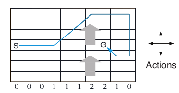
The grid world is represented as a 7 x 10 matrix of states. In the middle region the next states are shifted upward by wind (the strength in number of squares is given below each column). For example, if the agent is one cell to the right of the goal, then the action left takes the agent to the cell just above the goal.

No discounting is used (i.e., \gamma = 1).

References

Richard S. Sutton and Andrew G. Barto (2018). Reinforcement Learning: An Introduction Second Edition, MIT Press, Cambridge, MA.

See Also

Other MDP_examples: Cliff_walking, DynaMaze, MDP(), Maze

Other gridworld: Cliff_walking, DynaMaze, Maze, gridworld

Examples

data(Windy_gridworld)
Windy_gridworld

gridworld_matrix(Windy_gridworld)
gridworld_matrix(Windy_gridworld, what = "labels")

# The Goal is an absorbing state 
which(absorbing_states(Windy_gridworld))

# visualize the transition graph
gridworld_plot_transition_graph(Windy_gridworld, 
  vertex.size = 10, vertex.label = NA)

# solve using value iteration
sol <- solve_MDP(Windy_gridworld) 
sol
policy(sol)
gridworld_plot_policy(sol)

Access to Parts of the Model Description

Description

Functions to provide uniform access to different parts of the POMDP/MDP problem description.

Usage

start_vector(x)

normalize_POMDP(
  x,
  sparse = TRUE,
  trans_start = FALSE,
  trans_function = TRUE,
  trans_keyword = FALSE
)

normalize_MDP(
  x,
  sparse = TRUE,
  trans_start = FALSE,
  trans_function = TRUE,
  trans_keyword = FALSE
)

reward_matrix(
  x,
  action = NULL,
  start.state = NULL,
  end.state = NULL,
  observation = NULL,
  episode = NULL,
  epoch = NULL,
  sparse = FALSE
)

reward_val(
  x,
  action,
  start.state,
  end.state = NULL,
  observation = NULL,
  episode = NULL,
  epoch = NULL
)

transition_matrix(
  x,
  action = NULL,
  start.state = NULL,
  end.state = NULL,
  episode = NULL,
  epoch = NULL,
  sparse = FALSE,
  trans_keyword = TRUE
)

transition_val(x, action, start.state, end.state, episode = NULL, epoch = NULL)

observation_matrix(
  x,
  action = NULL,
  end.state = NULL,
  observation = NULL,
  episode = NULL,
  epoch = NULL,
  sparse = FALSE,
  trans_keyword = TRUE
)

observation_val(
  x,
  action,
  end.state,
  observation,
  episode = NULL,
  epoch = NULL
)

Arguments

Details

Several parts of the POMDP/MDP description can be defined in different ways. In particular, the fields transition_prob, observation_prob, reward, and start can be defined using matrices, data frames, keywords, or functions. See POMDP for details. The functions provided here, provide unified access to the data in these fields to make writing code easier.

Transition Probabilities T(s'|s,a)

transition_matrix() accesses the transition model. The complete model is a list with one element for each action. Each element contains a states x states matrix with s (start.state) as rows and s' (end.state) as columns. Matrices with a density below 50% can be requested in sparse format (as a Matrix::dgCMatrix).

Observation Probabilities O(o|s',a)

observation_matrix() accesses the observation model. The complete model is a list with one element for each action. Each element contains a states x observations matrix with s (start.state) as rows and o (observation) as columns. Matrices with a density below 50% can be requested in sparse format (as a Matrix::dgCMatrix)

Reward R(s,s',o,a)

reward_matrix() accesses the reward model. The preferred representation is a data.frame with the columns action, start.state, end.state, observation, and value. This is a sparse representation. The dense representation is a list of lists of matrices. The list levels are a (action) and s (start.state). The matrices have rows representing s' (end.state) and columns representing o (observations). The reward structure cannot be efficiently stored using a standard sparse matrix since there might be a fixed cost for each action resulting in no entries with 0.

Initial Belief

start_vector() translates the initial probability vector description into a numeric vector.

Convert the Complete POMDP Description into a consistent form

normalize_POMDP() returns a new POMDP definition where transition_prob, observations_prob, reward, and start are normalized.

Also, states, actions, and observations are ordered as given in the problem definition to make safe access using numerical indices possible. Normalized POMDP descriptions can be used in custom code that expects consistently a certain format.

Value

A list or a list of lists of matrices.

Author(s)

Michael Hahsler

See Also

Other POMDP: MDP2POMDP, POMDP(), actions(), add_policy(), plot_belief_space(), projection(), reachable_and_absorbing, regret(), sample_belief_space(), simulate_POMDP(), solve_POMDP(), solve_SARSOP(), transition_graph(), update_belief(), value_function(), write_POMDP()

Other MDP: MDP(), MDP2POMDP, MDP_policy_functions, actions(), add_policy(), gridworld, reachable_and_absorbing, regret(), simulate_MDP(), solve_MDP(), transition_graph(), value_function()

Examples

data("Tiger")

# List of |A| transition matrices. One per action in the from start.states x end.states
Tiger$transition_prob
transition_matrix(Tiger)
transition_val(Tiger, action = "listen", start.state = "tiger-left", end.state = "tiger-left")

# List of |A| observation matrices. One per action in the from states x observations
Tiger$observation_prob
observation_matrix(Tiger)
observation_val(Tiger, action = "listen", end.state = "tiger-left", observation = "tiger-left")

# List of list of reward matrices. 1st level is action and second level is the
#  start state in the form end state x observation
Tiger$reward
reward_matrix(Tiger)
reward_matrix(Tiger, sparse = TRUE)
reward_matrix(Tiger, action = "open-right", start.state = "tiger-left", end.state = "tiger-left",
  observation = "tiger-left")

# Translate the initial belief vector
Tiger$start
start_vector(Tiger)

# Normalize the whole model
Tiger_norm <- normalize_POMDP(Tiger)
Tiger_norm$transition_prob

## Visualize transition matrix for action 'open-left'
plot_transition_graph(Tiger)

## Use a function for the Tiger transition model
trans <- function(action, end.state, start.state) {
  ## listen has an identity matrix
  if (action == 'listen')
    if (end.state == start.state) return(1)
    else return(0)

  # other actions have a uniform distribution
  return(1/2)
}

Tiger$transition_prob <- trans

# transition_matrix evaluates the function
transition_matrix(Tiger)

Available Actions

Description

Determine the set of actions available in a state.

Usage

actions(x, state)

Arguments

Details

Unavailable actions are modeled here a actions that have an immediate reward of -Inf in the reward function.

Value

a character vector with the available actions.

a vector with the available actions.

Author(s)

Michael Hahsler

See Also

Other MDP: MDP(), MDP2POMDP, MDP_policy_functions, accessors, add_policy(), gridworld, reachable_and_absorbing, regret(), simulate_MDP(), solve_MDP(), transition_graph(), value_function()

Other POMDP: MDP2POMDP, POMDP(), accessors, add_policy(), plot_belief_space(), projection(), reachable_and_absorbing, regret(), sample_belief_space(), simulate_POMDP(), solve_POMDP(), solve_SARSOP(), transition_graph(), update_belief(), value_function(), write_POMDP()

Examples

data(RussianTiger)

# The normal actions are "listen", "open-left", and "open-right".
# In the state "done" only the action "nothing" is available. 

actions(RussianTiger, state = "tiger-left")
actions(RussianTiger, state = "tiger-right")
actions(RussianTiger, state = "done")

Add a Policy to a POMDP Problem Description

Description

Add a policy to a POMDP problem description allows the user to test policies on modified problem descriptions or to test manually created policies.

Usage

add_policy(model, policy)

Arguments

Value

The model description with the added policy.

Author(s)

Michael Hahsler

See Also

Other POMDP: MDP2POMDP, POMDP(), accessors, actions(), plot_belief_space(), projection(), reachable_and_absorbing, regret(), sample_belief_space(), simulate_POMDP(), solve_POMDP(), solve_SARSOP(), transition_graph(), update_belief(), value_function(), write_POMDP()

Other MDP: MDP(), MDP2POMDP, MDP_policy_functions, accessors, actions(), gridworld, reachable_and_absorbing, regret(), simulate_MDP(), solve_MDP(), transition_graph(), value_function()

Examples

data(Tiger)

sol <- solve_POMDP(Tiger)
sol

# Example 1: Use the solution policy on a changed POMDP problem
#            where listening is perfect and simulate the expected reward

perfect_Tiger <- Tiger
perfect_Tiger$observation_prob <- list(
  listen = diag(1, length(perfect_Tiger$states), 
    length(perfect_Tiger$observations)), 
  `open-left` = "uniform",
  `open-right` = "uniform"
)

sol_perfect <- add_policy(perfect_Tiger, sol)
sol_perfect

simulate_POMDP(sol_perfect, n = 1000)$avg_reward

# Example 2: Handcraft a policy and apply it to the Tiger problem

# original policy
policy(sol)
plot_value_function(sol)
plot_belief_space(sol)

# create a policy manually where the agent opens a door at a believe of 
#  roughly 2/3 (note the alpha vectors do not represent 
#  a valid value function)
p <- list(
data.frame(
  `tiger-left` = c(1, 0, -2),
  `tiger-right` = c(-2, 0, 1), 
  action = c("open-right", "listen", "open-left"),
  check.names = FALSE
))
p

custom_sol <- add_policy(Tiger, p)
custom_sol

policy(custom_sol)
plot_value_function(custom_sol)
plot_belief_space(custom_sol)

simulate_POMDP(custom_sol, n = 1000)$avg_reward

Default Colors for Visualization in Package pomdp

Description

Default discrete and continuous colors used in pomdp for states (nodes), beliefs and values.

Usage

colors_discrete(n, col = NULL)

colors_continuous(val, col = NULL)

Arguments

Value

colors_discrete() returns a color palette and colors_continuous() returns the colors associated with the supplied values.

Examples

colors_discrete(5)

colors_continuous(runif(10))

Estimate the Belief for Policy Graph Nodes

Description

Estimate a belief for each alpha vector (segment of the value function) which represents a node in the policy graph.

Usage

estimate_belief_for_nodes(
  x,
  method = "auto",
  belief = NULL,
  verbose = FALSE,
  ...
)

Arguments

Details

estimate_belief_for_nodes() can estimate the belief in several ways:

1. Use belief points explored by the solver. Some solvers return explored belief points. We assign the belief points to the nodes and average each nodes belief.

2. Follow trajectories (breadth first) till all policy graph nodes have been visited and return the encountered belief. This implementation returns the first (i.e., shallowest) belief point that is encountered is used and no averaging is performed. parameter n can be used to limit the number of nodes searched.

3. Sample a large set of possible belief points, assigning them to the nodes and then averaging the belief over the points assigned to each node. This will return a central belief for the node. Additional parameters like method and the sample size n are passed on to sample_belief_space(). If no belief point is generated for a segment, then a warning is produced. In this case, the number of sampled points can be increased.

Notes:

• Each method may return a different answer. The only thing that is guaranteed is that the returned belief falls in the range where the value function segment is maximal.

• If some nodes not belief points are sampled, or the node is not reachable from the initial belief, then a vector with all NaNs will be returned with a warning.

Value

returns a list with matrices with a belief for each policy graph node. The list elements are the epochs and converged solutions only have a single element.

See Also

Other policy: optimal_action(), plot_belief_space(), plot_policy_graph(), policy(), policy_graph(), projection(), reward(), solve_POMDP(), solve_SARSOP(), value_function()

Examples

data("Tiger")

# Infinite horizon case with converged solution
sol <- solve_POMDP(model = Tiger, method = "grid")
sol

# default method auto uses the belief points used in the algorithm (if available).
estimate_belief_for_nodes(sol, verbose = TRUE)

# use belief points obtained from trajectories  
estimate_belief_for_nodes(sol, method = "trajectories", verbose = TRUE)

# use a random uniform sample 
estimate_belief_for_nodes(sol, method = "random", verbose = TRUE)

# Finite horizon example with three epochs. 
sol <- solve_POMDP(model = Tiger, horizon = 3)
sol
estimate_belief_for_nodes(sol)

Helper Functions for Gridworld MDPs

Description

Helper functions for gridworld MDPs to convert between state names and gridworld positions, and for visualizing policies.

Usage

gridworld_init(
  dim,
  action_labels = c("up", "right", "down", "left"),
  unreachable_states = NULL,
  absorbing_states = NULL,
  labels = NULL
)

gridworld_maze_MDP(
  dim,
  start,
  goal,
  walls = NULL,
  action_labels = c("up", "right", "down", "left"),
  goal_reward = 1,
  step_cost = 0,
  restart = FALSE,
  discount = 0.9,
  horizon = Inf,
  info = NULL,
  name = NA
)

gridworld_s2rc(s)

gridworld_rc2s(rc)

gridworld_matrix(model, epoch = 1L, what = "states")

gridworld_plot_policy(
  model,
  epoch = 1L,
  actions = "character",
  states = FALSE,
  labels = TRUE,
  absorbing_state_action = FALSE,
  main = NULL,
  cex = 1,
  offset = 0.5,
  lines = TRUE,
  ...
)

gridworld_plot_transition_graph(
  x,
  hide_unreachable_states = TRUE,
  remove.loops = TRUE,
  vertex.color = "gray",
  vertex.shape = "square",
  vertex.size = 10,
  vertex.label = NA,
  edge.arrow.size = 0.3,
  margin = 0.2,
  main = NULL,
  ...
)

gridworld_animate(x, method, n, zlim = NULL, ...)

Arguments

Details

Gridworlds are implemented with state names s(row,col), where row and col are locations in the matrix representing the gridworld. The actions are "up", "right", "down", and "left".

gridworld_init() initializes a new gridworld creating a matrix of states with the given dimensions. Other action names can be specified, but they must have the same effects in the same order as above. Unreachable states (walls) and absorbing state can be defined. This information can be used to build a custom gridworld MDP.

Several helper functions are provided to use states, look at the state layout, and plot policies on the gridworld.

gridworld_maze_MDP() helps to easily define maze-like gridworld MDPs. By default, the goal state is absorbing, but with restart = TRUE, the agent restarts the problem at the start state every time it reaches the goal and receives the reward. Note that this implies that the goal state itself becomes unreachable.

gridworld_animate() applies algorithms from solve_MDP() iteration by iteration and visualized the state utilities. This helps to understand how the algorithms work.

See Also

Other gridworld: Cliff_walking, DynaMaze, Maze, Windy_gridworld

Other MDP: MDP(), MDP2POMDP, MDP_policy_functions, accessors, actions(), add_policy(), reachable_and_absorbing, regret(), simulate_MDP(), solve_MDP(), transition_graph(), value_function()

Examples

# Defines states, actions and a transition model for a standard gridworld
gw <- gridworld_init(dim = c(7,7),
                unreachable_states = c("s(2,2)", "s(7,3)", "s(3,6)"),
                absorbing_states = "s(4,4)",
                labels = list("s(4,4)" = "Black Hole")
                )

gw$states
gw$actions
gw$info

# display the state labels in the gridworld
gridworld_matrix(gw)
gridworld_matrix(gw, what = "label")
gridworld_matrix(gw, what = "reachable")
gridworld_matrix(gw, what = "absorbing")

# a transition function for regular moves in the gridworld is provided
gw$transition_prob("right", "s(1,1)", "s(1,2)")
gw$transition_prob("right", "s(2,1)", "s(2,2)")  ### we cannot move into an unreachable state
gw$transition_prob("right", "s(2,1)", "s(2,1)")  ### but the agent stays in place

# convert between state names and row/column indices
gridworld_s2rc("s(1,1)")
gridworld_rc2s(c(1,1))

# The information in gw can be used to build a custom MDP.

# We modify the standard transition function so there is a 50% chance that
# you will get sucked into the black hole from the adjacent squares.
trans_black_hole <- function(action = NA, start.state = NA, end.state = NA) {
  # ignore the action next to the black hole
  if (start.state %in% c("s(3,3)", "s(3,4)", "s(3,5)", "s(4,3)", "s(4,5)",
                         "s(5,3)", "s(5,4)", "s(5,5)")) {
        if(end.state == "s(4,4)")
            return(.5)
        else
            return(gw$transition_prob(action, start.state, end.state) * .5)
  }

  # use the standard gridworld movement
  gw$transition_prob(action, start.state, end.state)
}

black_hole <- MDP(states = gw$states,
  actions = gw$actions,
  transition_prob = trans_black_hole,
  reward = rbind(R_(value = +1), R_(end.state = "s(4,4)", value = -100)),
  info = gw$info,
  name = "Black hole"
  )

black_hole

gridworld_plot_transition_graph(black_hole)

# solve the problem
sol <- solve_MDP(black_hole)
gridworld_matrix(sol, what = "values")
gridworld_plot_policy(sol)
# the optimal policy is to fly around, but avoid the black hole.

# Build a Maze: The Dyna Maze from Chapter 8 in the RL book

DynaMaze <- gridworld_maze_MDP(
                dim = c(6,9),
                start = "s(3,1)",
                goal = "s(1,9)",
                walls = c("s(2,3)", "s(3,3)", "s(4,3)",
                          "s(5,6)",
                          "s(1,8)", "s(2,8)", "s(3,8)"),
                restart = TRUE,
                discount = 0.95,
                name = "Dyna Maze",
                )
DynaMaze

gridworld_matrix(DynaMaze)
gridworld_matrix(DynaMaze, what = "labels")

gridworld_plot_transition_graph(DynaMaze)
# Note that the problems resets if the goal state would be reached.

sol <- solve_MDP(DynaMaze)

gridworld_matrix(sol, what = "values")
gridworld_matrix(sol, what = "actions")
gridworld_plot_policy(sol)
gridworld_plot_policy(sol, actions = "label", cex = 1, states = FALSE)

# visualize the first 3 iterations of value iteration
gridworld_animate(DynaMaze, method = "value", n = 3)

Optimal action for a belief

Description

Determines the optimal action for a policy (solved POMDP) for a given belief at a given epoch.

Usage

optimal_action(model, belief = NULL, epoch = 1)

Arguments

Value

The name of the optimal action.

Author(s)

Michael Hahsler

See Also

Other policy: estimate_belief_for_nodes(), plot_belief_space(), plot_policy_graph(), policy(), policy_graph(), projection(), reward(), solve_POMDP(), solve_SARSOP(), value_function()

Examples

data("Tiger")
Tiger

sol <- solve_POMDP(model = Tiger)

# these are the states
sol$states

# belief that tiger is to the left
optimal_action(sol, c(1, 0))
optimal_action(sol, "tiger-left")

# belief that tiger is to the right
optimal_action(sol, c(0, 1))
optimal_action(sol, "tiger-right")

# belief is 50/50
optimal_action(sol, c(.5, .5))
optimal_action(sol, "uniform")

# the POMDP is converged, so all epoch give the same result.
optimal_action(sol, "tiger-right", epoch = 10)

Plot a 2D or 3D Projection of the Belief Space

Description

Plots the optimal action, the node in the policy graph or the reward for a given set of belief points on a line (2D) or on a ternary plot (3D). If no points are given, points are sampled using a regular arrangement or randomly from the (projected) belief space.

Usage

plot_belief_space(
  model,
  projection = NULL,
  epoch = 1,
  sample = "regular",
  n = 100,
  what = c("action", "pg_node", "reward"),
  legend = TRUE,
  pch = 20,
  col = NULL,
  jitter = 0,
  oneD = TRUE,
  ...
)

Arguments

Value

Returns invisibly the sampled points.

Author(s)

Michael Hahsler

See Also

Other policy: estimate_belief_for_nodes(), optimal_action(), plot_policy_graph(), policy(), policy_graph(), projection(), reward(), solve_POMDP(), solve_SARSOP(), value_function()

Other POMDP: MDP2POMDP, POMDP(), accessors, actions(), add_policy(), projection(), reachable_and_absorbing, regret(), sample_belief_space(), simulate_POMDP(), solve_POMDP(), solve_SARSOP(), transition_graph(), update_belief(), value_function(), write_POMDP()

Examples

# two-state POMDP
data("Tiger")
sol <- solve_POMDP(Tiger)

plot_belief_space(sol)
plot_belief_space(sol, oneD = FALSE)
plot_belief_space(sol, n = 10)
plot_belief_space(sol, n = 100, sample = "random")

# plot the belief points used by the grid-based solver
plot_belief_space(sol, sample = sol $solution$belief_points_solver)

# plot different measures
plot_belief_space(sol, what = "pg_node")
plot_belief_space(sol, what = "reward")

# three-state POMDP
# Note: If the plotting region is too small then the legend might run into the plot
data("Three_doors")
sol <- solve_POMDP(Three_doors)
sol

# plotting needs the suggested package Ternary
if ("Ternary" %in% installed.packages()) {
plot_belief_space(sol)
plot_belief_space(sol, n = 10000)
plot_belief_space(sol, what = "reward", sample = "random", n = 1000)
plot_belief_space(sol, what = "pg_node", n = 10000)

# holding tiger-left constant at .5 follows this line in the ternary plot 
Ternary::TernaryLines(list(c(.5, 0, .5), c(.5, .5, 0)), col = "black", lty = 2)
# we can plot the projection for this line 
plot_belief_space(sol, what = "pg_node", n = 1000, projection = c("tiger-left" = .5))

# plot the belief points used by the grid-based solver
plot_belief_space(sol, sample = sol$solution$belief_points_solver, what = "pg_node")

# plot the belief points obtained using simulated trajectories with an epsilon-greedy policy.
# Note that we only use n = 50 to save time.
plot_belief_space(sol, 
  sample = simulate_POMDP(sol, n = 50, horizon = 100,
    epsilon = 0.1, return_beliefs = TRUE)$belief_states)
}

# plot a 3-state belief space using ggtern (ggplot2)
## Not run: 
library(ggtern)
samp <- sample_belief_space(sol, n = 1000)
df <- cbind(as.data.frame(samp), reward_node_action(sol, belief = samp))
df$pg_node <- factor(df$pg_node)

ggtern(df, aes(x = `tiger-left`, y = `tiger-center`, z = `tiger-right`)) +
  geom_point(aes(color = pg_node), size = 2)

ggtern(df, aes(x = `tiger-left`, y = `tiger-center`, z = `tiger-right`)) +
  geom_point(aes(color = action), size = 2)

ggtern(df, aes(x = `tiger-left`, y = `tiger-center`, z = `tiger-right`)) +
  geom_point(aes(color = reward), size = 2)

## End(Not run)

POMDP Plot Policy Graphs

Description

The function plots the POMDP policy graph for converged POMDP solution and the policy tree for a finite-horizon solution.

Usage

plot_policy_graph(
  x,
  belief = NULL,
  engine = c("igraph", "visNetwork"),
  show_belief = TRUE,
  state_col = NULL,
  legend = TRUE,
  simplify_observations = TRUE,
  remove_unreachable_nodes = TRUE,
  ...
)

curve_multiple_directed(graph, start = 0.3)

Arguments

Details

The policy graph returned by policy_graph() can be directly plotted. plot_policy_graph() uses policy_graph() to get the policy graph and produces an improved visualization (a legend, tree layout for finite-horizon solutions, better edge curving, etc.). It also offers an interactive visualization using visNetwork::visIgraph().

Each policy graph node is represented by an alpha vector specifying a hyper plane segment. The convex hull of the set of hyperplanes represents the the value function. The policy specifies for each node an optimal action which is printed together with the node ID inside the node. The arcs are labeled with observations. Infinite-horizon converged solutions from a single policy graph. For finite-horizon solution a policy tree is produced. The levels of the tree and the first number in the node label represent the epochs.

For better visualization, we provide a few features:

• Show Belief, belief color and legend: A pie chart (or the color) in each node can be used represent an example of the belief that the agent has if it is in this node. This can help with interpreting the policy graph. The belief is obtained by calling estimate_belief_for_nodes().

• Simplify observations: In some cases, two observations can lead to the same node resulting in two parallel edges. These edges can be collapsed into one labels with the observations.

• Remove unreachable nodes: Many algorithms produce unused policy graph nodes which can be filtered to produce a smaller tree structure of actually used nodes. Non-converged policies depend on the initial belief and if an initial belief is specified, then different nodes will be filtered and the tree will look different.

These improvements can be disabled using parameters.

Auxiliary function

curve_multiple_directed() is a helper function for plotting igraph graphs similar to igraph::curve_multiple() but it also adds curvature to parallel edges that point in opposite directions.

Value

returns invisibly what the plotting engine returns.

See Also

Other policy: estimate_belief_for_nodes(), optimal_action(), plot_belief_space(), policy(), policy_graph(), projection(), reward(), solve_POMDP(), solve_SARSOP(), value_function()

Examples

data("Tiger")

### Policy graphs for converged solutions
sol <- solve_POMDP(model = Tiger)
sol

policy_graph(sol)

## visualization
plot_policy_graph(sol)

## use a different graph layout (circle and manual; needs igraph)
library("igraph")
plot_policy_graph(sol, layout = layout.circle)
plot_policy_graph(sol, layout = rbind(c(1,1), c(1,-1), c(0,0), c(-1,-1), c(-1,1)), margin = .2)
plot_policy_graph(sol,
  layout = rbind(c(1,0), c(.5,0), c(0,0), c(-.5,0), c(-1,0)), rescale = FALSE,
  vertex.size = 15, edge.curved = 2,
  main = "Tiger Problem")

## hide labels, beliefs and legend
plot_policy_graph(sol, show_belief = FALSE, edge.label = NA, vertex.label = NA, legend = FALSE)

## custom larger vertex labels (A, B, ...)
plot_policy_graph(sol,
  vertex.label = LETTERS[1:nrow(policy(sol))],
  vertex.size = 60,
  vertex.label.cex = 2,
  edge.label.cex = .7,
  vertex.label.color = "white")

## plotting the igraph object directly
pg <- policy_graph(sol, show_belief = TRUE, 
  simplify_observations = TRUE, remove_unreachable_nodes = TRUE)

## (e.g., using a tree layout)
plot(pg, layout = layout_as_tree(pg, root = 3, mode = "out"))

## change labels (abbreviate observations and use only actions to label the vertices)
plot(pg,
  edge.label = abbreviate(E(pg)$label),
  vertex.label = V(pg)$action,
  vertex.size = 20)

## use action to color vertices (requires a graph without a belief pie chart) 
##    and color edges to represent observations.
pg <- policy_graph(sol, show_belief = FALSE, 
  simplify_observations = TRUE, remove_unreachable_nodes = TRUE)

plot(pg,
  vertex.label = NA,
  vertex.color = factor(V(pg)$action),
  vertex.size = 20,
  edge.color = factor(E(pg)$observation),
  edge.curved = .1
  )

acts <- levels(factor(V(pg)$action))
legend("topright", legend = acts, title = "action",
  col = igraph::categorical_pal(length(acts)), pch = 15)
obs <- levels(factor(E(pg)$observation))
legend("bottomright", legend = obs, title = "observation",
  col = igraph::categorical_pal(length(obs)), lty = 1) 

## plot interactive graphs using the visNetwork library.
## Note: the pie chart representation is not available, but colors are used instead.
plot_policy_graph(sol, engine = "visNetwork")

## add smooth edges and a layout (note, engine can be abbreviated)
plot_policy_graph(sol, engine = "visNetwork", layout = "layout_in_circle", smooth = TRUE)


### Policy trees for finite-horizon solutions
sol <- solve_POMDP(model = Tiger, horizon = 4, method = "incprune")

policy_graph(sol)

plot_policy_graph(sol)
# Note: the first number in the node id is the epoch.

# plot the policy tree for an initial belief of 90% that the tiger is to the left
plot_policy_graph(sol, belief = c(0.9, 0.1))

# Plotting a larger graph (see ? igraph.plotting for plotting options)
sol <- solve_POMDP(model = Tiger, horizon = 10, method = "incprune")

plot_policy_graph(sol, edge.arrow.size = .1,
  vertex.label.cex = .5, edge.label.cex = .5)

plot_policy_graph(sol, engine = "visNetwork")

Extract the Policy from a POMDP/MDP

Description

Extracts the policy from a solved POMDP/MDP.

Usage

policy(x, drop = TRUE)

Arguments

Details

A list (one entry per epoch) with the optimal policy. For converged, infinite-horizon problems solutions, a list with only the converged solution is produced. For a POMDP, the policy is a data.frame consisting of:

• Part 1: The alpha vectors for the belief states (defines also the utility of the belief). The columns have the names of states.

• Part 2: The last column named action contains the prescribed action.

For an MDP, the policy is a data.frame with columns for:

• state: The state.

• U: The state's value (discounted expected utility U) if the policy is followed

• action: The prescribed action.

Value

A list with the policy for each epoch. Converged policies have only one element. If drop = TRUE then the policy is returned without a list.

Author(s)

Michael Hahsler

See Also

Other policy: estimate_belief_for_nodes(), optimal_action(), plot_belief_space(), plot_policy_graph(), policy_graph(), projection(), reward(), solve_POMDP(), solve_SARSOP(), value_function()

Examples

data("Tiger")

# Infinite horizon
sol <- solve_POMDP(model = Tiger)
sol

# policy with value function, optimal action and transitions for observations.
policy(sol)
plot_value_function(sol)

# Finite horizon (we use incremental pruning because grid does not converge)
sol <- solve_POMDP(model = Tiger, method = "incprune", 
  horizon = 3, discount = 1)
sol

policy(sol)
# Note: We see that it is initially better to listen till we make 
#       a decision in the final epoch.

# MDP policy
data(Maze)

sol <- solve_MDP(Maze)

policy(sol)

POMDP Policy Graphs

Description

The function creates a POMDP policy graph for converged POMDP solution and the policy tree for a finite-horizon solution. The graph is represented as an igraph object.

Usage

policy_graph(
  x,
  belief = NULL,
  show_belief = FALSE,
  state_col = NULL,
  simplify_observations = FALSE,
  remove_unreachable_nodes = FALSE,
  ...
)

Arguments

Details

Each policy graph node is represented by an alpha vector specifying a hyper plane segment. The convex hull of the set of hyperplanes represents the the value function. The policy specifies for each node an optimal action which is printed together with the node ID inside the node. The arcs are labeled with observations. Infinite-horizon converged solutions from a single policy graph. For finite-horizon solution a policy tree is produced. The levels of the tree and the first number in the node label represent the epochs.

The parameters show_belief, remove_unreachable_nodes, and simplify_observations are used by plot_policy_graph() (see there for details) to reduce clutter and make the visualization more readable. These options are disabled by default for policy_graph().

Value

returns the policy graph as an igraph object.

See Also

Other policy: estimate_belief_for_nodes(), optimal_action(), plot_belief_space(), plot_policy_graph(), policy(), projection(), reward(), solve_POMDP(), solve_SARSOP(), value_function()

Examples

data("Tiger")

### Policy graphs for converged solutions
sol <- solve_POMDP(model = Tiger)
sol

policy_graph(sol)

## visualization
plot_policy_graph(sol)

### Policy trees for finite-horizon solutions
sol <- solve_POMDP(model = Tiger, horizon = 4, method = "incprune")

policy_graph(sol)
plot_policy_graph(sol)
# Note: the first number in the node id is the epoch.

Defining a Belief Space Projection

Description

High dimensional belief spaces can be projected to lower dimension. This is useful for visualization and to analyze the belief space and value functions. This definition is used by functions like plot_belief_space(), plot_value_function(), and sample_belief_space().

Usage

projection(x = NULL, model)

Arguments

Details

The belief space is $n-1$ dimensional, were $n$ is the number of states. Note: it is n-1 dimensional since the probabilities need to add up to 1. A projection fixes the belief value for a set of states. For example, for a 4-state POMDP (s1, s2, s3, s4), we can project the belief space on s1 and s2 by holding s3 and s4 constant which is represented by the vector c(s1 = NA, s2 = NA, s3 = 0, s4 = .1). We use NA to represent that the values are not fixed and the value that the other dimensions are held constant.

We provide several ways to specify a projection:

• A vector with values for all dimensions. NAs are used for the dimension projected on. This is the canonical form used in this package. Example: c(NA, NA, 0, .1)

• A named vector with just the dimensions held constant. Example: c(s3 = 0, s4 = .1)

• A vector of state names to project on. All other dimensions are held constant at 0. Example: c("s1", "s2")

• A vector with indices of the states to project on. All other dimensions are held constant at 0. Example: c(1, 2)

Value

a canonical description of the projection.

Author(s)

Michael Hahsler

See Also

Other policy: estimate_belief_for_nodes(), optimal_action(), plot_belief_space(), plot_policy_graph(), policy(), policy_graph(), reward(), solve_POMDP(), solve_SARSOP(), value_function()

Other POMDP: MDP2POMDP, POMDP(), accessors, actions(), add_policy(), plot_belief_space(), reachable_and_absorbing, regret(), sample_belief_space(), simulate_POMDP(), solve_POMDP(), solve_SARSOP(), transition_graph(), update_belief(), value_function(), write_POMDP()

Examples

model <- POMDP(
 states = 4,
 actions = 2,
 observations = 2,
 transition_prob = list("identity","identity"),
 observation_prob = list("uniform","uniform"),
 reward = rbind(R_(value = 1))
)

projection(NULL, model = model)
projection(1:2, model = model)
projection(c("s2", "s3"), model = model)
projection(c(1,4), model = model)
projection(c(s2 = .4, s3 = .2), model = model)
projection(c(s1 = .1, s2 = NA, s3 = NA, s4 = .3), model = model)

Reachable and Absorbing States

Description

Find reachable and absorbing states in the transition model.

Usage

reachable_states(x, states = NULL)

absorbing_states(x, states = NULL)

remove_unreachable_states(x)

Arguments

Details

The function reachable_states() checks if states are reachable using the transition model.

The function absorbing_states() checks if a state or a set of states are absorbing (terminal states) with a zero reward (or -Inf for unavailable actions). If no states are specified (states = NULL), then all model states are checked. This information can be used in simulations to end an episode.

The function remove_unreachable_states() simplifies a model by removing unreachable states.

Value

reachable_states() returns a logical vector indicating if the states are reachable.

absorbing_states() returns a logical vector indicating if the states are absorbing (terminal).

the model with all unreachable states removed

Author(s)

Michael Hahsler

See Also

Other MDP: MDP(), MDP2POMDP, MDP_policy_functions, accessors, actions(), add_policy(), gridworld, regret(), simulate_MDP(), solve_MDP(), transition_graph(), value_function()

Other POMDP: MDP2POMDP, POMDP(), accessors, actions(), add_policy(), plot_belief_space(), projection(), regret(), sample_belief_space(), simulate_POMDP(), solve_POMDP(), solve_SARSOP(), transition_graph(), update_belief(), value_function(), write_POMDP()

Examples

data(Maze)

gridworld_matrix(Maze, what = "label")

# the states marked with +1 and -1 are absorbing
absorbing_states(Maze)
which(absorbing_states(Maze))

# all states in the model are reachable
reachable_states(Maze)
which(!reachable_states(Maze))

Calculate the Regret of a Policy

Description

Calculates the regret of a policy relative to a benchmark policy.

Usage

regret(policy, benchmark, start = NULL)

Arguments

Details

Regret is defined as V^{\pi^*}(s_0) - V^{\pi}(s_0) with V^\pi representing the expected long-term state value (represented by the value function) given the policy \pi and the start state s_0. For POMDPs the start state is the start belief b_0.

Note that for regret usually the optimal policy \pi^* is used as the benchmark. Since the optimal policy may not be known, regret relative to the best known policy can be used.

Value

the regret as a difference of expected long-term rewards.

Author(s)

Michael Hahsler

See Also

Other POMDP: MDP2POMDP, POMDP(), accessors, actions(), add_policy(), plot_belief_space(), projection(), reachable_and_absorbing, sample_belief_space(), simulate_POMDP(), solve_POMDP(), solve_SARSOP(), transition_graph(), update_belief(), value_function(), write_POMDP()

Other MDP: MDP(), MDP2POMDP, MDP_policy_functions, accessors, actions(), add_policy(), gridworld, reachable_and_absorbing, simulate_MDP(), solve_MDP(), transition_graph(), value_function()

Examples

data(Tiger)

sol_optimal <- solve_POMDP(Tiger)
sol_optimal

# perform exact value iteration for 10 epochs
sol_quick <- solve_POMDP(Tiger, method = "enum", horizon = 10)
sol_quick

regret(sol_quick, benchmark = sol_optimal)

Calculate the Reward for a POMDP Solution

Description

This function calculates the expected total reward for a POMDP solution given a starting belief state. The value is calculated using the value function stored in the POMDP solution. In addition, the policy graph node that represents the belief state and the optimal action can also be returned using reward_node_action().

Usage

reward(x, belief = NULL, epoch = 1, ...)

reward_node_action(x, belief = NULL, epoch = 1, ...)

Arguments

Details

The reward is typically calculated using the value function (alpha vectors) of the solution. If these are not available, then simulate_POMDP() is used instead with a warning.

Value

reward() returns a vector of reward values, one for each belief if a matrix is specified.

reward_node_action() returns a list with the components

Author(s)

Michael Hahsler

See Also

Other policy: estimate_belief_for_nodes(), optimal_action(), plot_belief_space(), plot_policy_graph(), policy(), policy_graph(), projection(), solve_POMDP(), solve_SARSOP(), value_function()

Examples

data("Tiger")
sol <- solve_POMDP(model = Tiger)

# if no start is specified, a uniform belief is used.
reward(sol)

# we have additional information that makes us believe that the tiger
# is more likely to the left.
reward(sol, belief = c(0.85, 0.15))

# we start with strong evidence that the tiger is to the left.
reward(sol, belief = "tiger-left")

# Note that in this case, the total discounted expected reward is greater
# than 10 since the tiger problem resets and another game staring with
# a uniform belief is played which produces additional reward.

# return reward, the initial node in the policy graph and the optimal action for
# two beliefs.
reward_node_action(sol, belief = rbind(c(.5, .5), c(.9, .1)))

# manually combining reward with belief space sampling to show the value function
# (color signifies the optimal action)
samp <- sample_belief_space(sol, n = 200)
rew <- reward_node_action(sol, belief = samp)
plot(rew$belief[,"tiger-right"], rew$reward, col = rew$action, ylim = c(0, 15))
legend(x = "top", legend = levels(rew$action), title = "action", col = 1:3, pch = 1)

# this is the piecewise linear value function from the solution
plot_value_function(sol, ylim = c(0, 10))

Round a stochastic vector or a row-stochastic matrix

Description

Rounds a vector such that the sum of 1 is preserved. Rounds a matrix such that each row sum up to 1. One entry is adjusted after rounding such that the rounding error is the smallest.

Usage

round_stochastic(x, digits = 7)

Arguments

Value

The rounded vector or matrix.

See Also

round

Examples

# regular rounding would not sum up to 1 
x <- c(0.333, 0.334, 0.333)

round_stochastic(x)
round_stochastic(x, digits = 2)
round_stochastic(x, digits = 1)
round_stochastic(x, digits = 0)


# round a stochastic matrix
m <- matrix(runif(15), ncol = 3)
m <- sweep(m, 1, rowSums(m), "/")

m
round_stochastic(m, digits = 2)
round_stochastic(m, digits = 1)
round_stochastic(m, digits = 0)

Sample from the Belief Space

Description

Sample points from belief space using a several sampling strategies.

Usage

sample_belief_space(model, projection = NULL, n = 1000, method = "random", ...)

Arguments

Details

The purpose of sampling from the belief space is to provide good coverage or to sample belief points that are more likely to be encountered (see trajectory method). The following sampling methods are available:

• 'random' samples uniformly sample from the projected belief space using the method described by Luc Devroye (1986). Sampling is be done in parallel after a foreach backend is registered.

• 'regular' samples points using a regularly spaced grid. This method is only available for projections on 2 or 3 states.

• "trajectories" returns the belief states encountered in n trajectories of length horizon starting at the model's initial belief. Thus it returns n x horizon belief states and will contain duplicates. Projection is not supported for trajectories. Additional arguments can include the simulation horizon and the start belief which are passed on to simulate_POMDP().

Value

Returns a matrix. Each row is a sample from the belief space.

Author(s)

Michael Hahsler

References

Luc Devroye, Non-Uniform Random Variate Generation, Springer Verlag, 1986.

See Also

Other POMDP: MDP2POMDP, POMDP(), accessors, actions(), add_policy(), plot_belief_space(), projection(), reachable_and_absorbing, regret(), simulate_POMDP(), solve_POMDP(), solve_SARSOP(), transition_graph(), update_belief(), value_function(), write_POMDP()

Examples

data("Tiger")

# random sampling can be done in parallel after registering a backend.
# doparallel::registerDoParallel()

sample_belief_space(Tiger, n = 5)
sample_belief_space(Tiger, n = 5, method = "regular")
sample_belief_space(Tiger, n = 1, horizon = 5, method = "trajectories")

# sample, determine the optimal action and calculate the expected reward for a solved POMDP
# Note: check.names = FALSE is used to preserve the `-` for the state names in the dataframe.
sol <- solve_POMDP(Tiger)
samp <- sample_belief_space(sol, n = 5, method = "regular")
data.frame(samp, action = optimal_action(sol,  belief = samp), 
  reward = reward(sol, belief = samp), check.names = FALSE)
  
# sample from a 3 state problem
data(Three_doors)
Three_doors

sample_belief_space(Three_doors, n = 5)
sample_belief_space(Three_doors, n = 5, projection = c(`tiger-left` = .1))

if ("Ternary" %in% installed.packages()) {
sample_belief_space(Three_doors, n = 9, method = "regular")
sample_belief_space(Three_doors, n = 9, method = "regular", projection = c(`tiger-left` = .1))
}

sample_belief_space(Three_doors, n = 1, horizon = 5, method = "trajectories")

Simulate Trajectories in a MDP

Description

Simulate trajectories through a MDP. The start state for each trajectory is randomly chosen using the specified belief. The belief is used to choose actions from an epsilon-greedy policy and then update the state.

Usage

simulate_MDP(
  model,
  n = 100,
  start = NULL,
  horizon = NULL,
  epsilon = NULL,
  delta_horizon = 0.001,
  return_trajectories = FALSE,
  engine = "cpp",
  verbose = FALSE,
  ...
)

Arguments

Details

A native R implementation is available (engine = 'r') and the default is a faster C++ implementation (engine = 'cpp').

Both implementations support parallel execution using the package foreach. To enable parallel execution, a parallel backend like doparallel needs to be available needs to be registered (see doParallel::registerDoParallel()). Note that small simulations are slower using parallelization. Therefore, C++ simulations with n * horizon less than 100,000 are always executed using a single worker.

Value

A list with elements:

• avg_reward: The average discounted reward.

• reward: Reward for each trajectory.

• action_cnt: Action counts.

• state_cnt: State counts.

• trajectories: A data.frame with the trajectories. Each row contains the episode id, the time step, the state s, the chosen action a, the reward r, and the next state s_prime. Trajectories are only returned for return_trajectories = TRUE.

Author(s)

Michael Hahsler

See Also

Other MDP: MDP(), MDP2POMDP, MDP_policy_functions, accessors, actions(), add_policy(), gridworld, reachable_and_absorbing, regret(), solve_MDP(), transition_graph(), value_function()

Examples

# enable parallel simulation 
# doParallel::registerDoParallel()

data(Maze)

# solve the POMDP for 5 epochs and no discounting
sol <- solve_MDP(Maze, discount = 1)
sol

# U in the policy is and estimate of the utility of being in a state when using the optimal policy.
policy(sol)
gridworld_matrix(sol, what = "action")

## Example 1: simulate 100 trajectories following the policy, 
#             only the final belief state is returned
sim <- simulate_MDP(sol, n = 100, horizon = 10, verbose = TRUE)
sim

# Note that all simulations start at s_1 and that the simulated avg. reward
# is therefore an estimate to the U value for the start state s_1.
policy(sol)[1,]

# Calculate proportion of actions taken in the simulation
round_stochastic(sim$action_cnt / sum(sim$action_cnt), 2)

# reward distribution
hist(sim$reward)

## Example 2: simulate starting following a uniform distribution over all
#             states and return all trajectories
sim <- simulate_MDP(sol, n = 100, start = "uniform", horizon = 10, 
  return_trajectories = TRUE)
head(sim$trajectories)   
  
# how often was each state visited?
table(sim$trajectories$s)

Simulate Trajectories Through a POMDP

Description

Simulate trajectories through a POMDP. The start state for each trajectory is randomly chosen using the specified belief. The belief is used to choose actions from the the epsilon-greedy policy and then updated using observations.

Usage

simulate_POMDP(
  model,
  n = 1000,
  belief = NULL,
  horizon = NULL,
  epsilon = NULL,
  delta_horizon = 0.001,
  digits = 7L,
  return_beliefs = FALSE,
  return_trajectories = FALSE,
  engine = "cpp",
  verbose = FALSE,
  ...
)

Arguments

Details

Simulates n trajectories. If no simulation horizon is specified, the horizon of finite-horizon problems is used. For infinite-horizon problems with \gamma < 1, the simulation horizon T is chosen such that the worst-case error is no more than \delta_\text{horizon}. That is

\gamma^T \frac{R_\text{max}}{\gamma} \le \delta_\text{horizon},

where R_\text{max} is the largest possible absolute reward value used as a perpetuity starting after T.

A native R implementation (engine = 'r') and a faster C++ implementation (engine = 'cpp') are available. Currently, only the R implementation supports multi-episode problems.

Both implementations support the simulation of trajectories in parallel using the package foreach. To enable parallel execution, a parallel backend like doparallel needs to be registered (see doParallel::registerDoParallel()). Note that small simulations are slower using parallelization. C++ simulations with n * horizon less than 100,000 are always executed using a single worker.

Value

A list with elements:

• avg_reward: The average discounted reward.

• action_cnt: Action counts.

• state_cnt: State counts.

• reward: Reward for each trajectory.

• belief_states: A matrix with belief states as rows.

• trajectories: A data.frame with the episode id, time, the state of the simulation (simulation_state), the id of the used alpha vector given the current belief (see belief_states above), the action a and the reward r.

Author(s)

Michael Hahsler

See Also

Other POMDP: MDP2POMDP, POMDP(), accessors, actions(), add_policy(), plot_belief_space(), projection(), reachable_and_absorbing, regret(), sample_belief_space(), solve_POMDP(), solve_SARSOP(), transition_graph(), update_belief(), value_function(), write_POMDP()

Examples

data(Tiger)

# solve the POMDP for 5 epochs and no discounting
sol <- solve_POMDP(Tiger, horizon = 5, discount = 1, method = "enum")
sol
policy(sol)

# uncomment the following line to register a parallel backend for simulation 
# (needs package doparallel installed)

# doParallel::registerDoParallel()
# foreach::getDoParWorkers()

## Example 1: simulate 100 trajectories
sim <- simulate_POMDP(sol, n = 100, verbose = TRUE)
sim

# calculate the percentage that each action is used in the simulation
round_stochastic(sim$action_cnt / sum(sim$action_cnt), 2)

# reward distribution
hist(sim$reward)


## Example 2: look at the belief states and the trajectories starting with 
#             an initial start belief.
sim <- simulate_POMDP(sol, n = 100, belief = c(.5, .5), 
  return_beliefs = TRUE, return_trajectories = TRUE)
head(sim$belief_states)
head(sim$trajectories)

# plot with added density (the x-axis is the probability of the second belief state)
plot_belief_space(sol, sample = sim$belief_states, jitter = 2, ylim = c(0, 6))
lines(density(sim$belief_states[, 2], bw = .02)); axis(2); title(ylab = "Density")


## Example 3: simulate trajectories for an unsolved POMDP which uses an epsilon of 1
#             (i.e., all actions are randomized). The simulation horizon for the 
#             infinite-horizon Tiger problem is calculated using delta_horizon. 
sim <- simulate_POMDP(Tiger, return_beliefs = TRUE, verbose = TRUE)
sim$avg_reward

hist(sim$reward, breaks = 20)

plot_belief_space(sol, sample = sim$belief_states, jitter = 2, ylim = c(0, 6))
lines(density(sim$belief_states[, 1], bw = .05)); axis(2); title(ylab = "Density")

Solve an MDP Problem

Description

Implementation of value iteration, modified policy iteration and other methods based on reinforcement learning techniques to solve finite state space MDPs.

Usage

solve_MDP(model, method = "value", ...)

solve_MDP_DP(
  model,
  method = "value_iteration",
  horizon = NULL,
  discount = NULL,
  N_max = 1000,
  error = 0.01,
  k_backups = 10,
  U = NULL,
  verbose = FALSE
)

solve_MDP_TD(
  model,
  method = "q_learning",
  horizon = NULL,
  discount = NULL,
  alpha = 0.5,
  epsilon = 0.1,
  N = 100,
  U = NULL,
  verbose = FALSE
)

Arguments

Details

Implemented are the following dynamic programming methods (following Russell and Norvig, 2010):

• Modified Policy Iteration starts with a random policy and iteratively performs a sequence of

  1. approximate policy evaluation (estimate the value function for the current policy using k_backups and function MDP_policy_evaluation()), and

  2. policy improvement (calculate a greedy policy given the value function). The algorithm stops when it converges to a stable policy (i.e., no changes between two iterations).

• Value Iteration starts with an arbitrary value function (by default all 0s) and iteratively updates the value function for each state using the Bellman equation. The iterations are terminated either after N_max iterations or when the solution converges. Approximate convergence is achieved for discounted problems (with \gamma < 1) when the maximal value function change for any state \delta is \delta \le error (1-\gamma) / \gamma. It can be shown that this means that no state value is more than error from the value in the optimal value function. For undiscounted problems, we use \delta \le error.

  The greedy policy is calculated from the final value function. Value iteration can be seen as policy iteration with truncated policy evaluation.

Note that the policy converges earlier than the value function.

Implemented are the following temporal difference control methods described in Sutton and Barto (2020). Note that the MDP transition and reward models are only used to simulate the environment for these reinforcement learning methods. The algorithms use a step size parameter \alpha (learning rate) for the updates and the exploration parameter \epsilon for the \epsilon-greedy policy.

If the model has absorbing states to terminate episodes, then no maximal episode length (horizon) needs to be specified. To make sure that the algorithm does finish in a reasonable amount of time, episodes are stopped after 10,000 actions with a warning. For models without absorbing states, a episode length has to be specified via horizon.

• Q-Learning is an off-policy temporal difference method that uses an \epsilon-greedy behavior policy and learns a greedy target policy.

• Sarsa is an on-policy method that follows and learns an \epsilon-greedy policy. The final \epsilon-greedy policy is converted into a greedy policy.

• Expected Sarsa: We implement an on-policy version that uses the expected value under the current policy for the update. It moves deterministically in the same direction as Sarsa moves in expectation. Because it uses the expectation, we can set the step size \alpha to large values and even 1.

Value

solve_MDP() returns an object of class POMDP which is a list with the model specifications (model), the solution (solution). The solution is a list with the elements:

• policy a list representing the policy graph. The list only has one element for converged solutions.

• converged did the algorithm converge (NA) for finite-horizon problems.

• delta final \delta (value iteration and infinite-horizon only)

• iterations number of iterations to convergence (infinite-horizon only)

Author(s)

Michael Hahsler

References

Russell, S., Norvig, P. (2021). Artificial Intelligence: A Modern Approach. Fourth edition. Prentice Hall.

Sutton, R. S., Barto, A. G. (2020). Reinforcement Learning: An Introduction. Second edition. The MIT Press.

See Also

Other solver: solve_POMDP(), solve_SARSOP()

Other MDP: MDP(), MDP2POMDP, MDP_policy_functions, accessors, actions(), add_policy(), gridworld, reachable_and_absorbing, regret(), simulate_MDP(), transition_graph(), value_function()

Examples

data(Maze)
Maze

# use value iteration
maze_solved <- solve_MDP(Maze, method = "value_iteration")
maze_solved
policy(maze_solved)

# plot the value function U
plot_value_function(maze_solved)

# Maze solutions can be visualized
gridworld_plot_policy(maze_solved)

# use modified policy iteration
maze_solved <- solve_MDP(Maze, method = "policy_iteration")
policy(maze_solved)

# finite horizon
maze_solved <- solve_MDP(Maze, method = "value_iteration", horizon = 3)
policy(maze_solved)
gridworld_plot_policy(maze_solved, epoch = 1)
gridworld_plot_policy(maze_solved, epoch = 2)
gridworld_plot_policy(maze_solved, epoch = 3)

# create a random policy where action n is very likely and approximate
#  the value function. We change the discount factor to .9 for this.
Maze_discounted <- Maze
Maze_discounted$discount <- .9
pi <- random_MDP_policy(Maze_discounted, 
        prob = c(n = .7, e = .1, s = .1, w = 0.1))
pi

# compare the utility function for the random policy with the function for the optimal
#  policy found by the solver.
maze_solved <- solve_MDP(Maze)

MDP_policy_evaluation(pi, Maze, k_backup = 100)
MDP_policy_evaluation(policy(maze_solved), Maze, k_backup = 100)

# Note that the solver already calculates the utility function and returns it with the policy
policy(maze_solved)

# Learn a Policy using Q-Learning
maze_learned <- solve_MDP(Maze, method = "q_learning", N = 100)
maze_learned

maze_learned$solution
policy(maze_learned)
plot_value_function(maze_learned)
gridworld_plot_policy(maze_learned)

Solve a POMDP Problem using pomdp-solver

Description

This function utilizes the C implementation of 'pomdp-solve' by Cassandra (2015) to solve problems that are formulated as partially observable Markov decision processes (POMDPs). The result is an optimal or approximately optimal policy.

Usage

solve_POMDP(
  model,
  horizon = NULL,
  discount = NULL,
  initial_belief = NULL,
  terminal_values = NULL,
  method = "grid",
  digits = 7,
  parameter = NULL,
  timeout = Inf,
  verbose = FALSE
)

solve_POMDP_parameter()

Arguments

Details

Parameters

solve_POMDP_parameter() displays available solver parameter options.

Horizon: Infinite-horizon POMDPs (horizon = Inf) converge to a single policy graph. Finite-horizon POMDPs result in a policy tree of a depth equal to the smaller of the horizon or the number of epochs to convergence. The policy (and the associated value function) are stored in a list by epoch. The policy for the first epoch is stored as the first element. Horizon can also be used to limit the number of epochs used for value iteration.

Precision: The POMDP solver uses various epsilon values to control precision for comparing alpha vectors to check for convergence, and solving LPs. Overall precision can be changed using parameter = list(epsilon = 1e-3).

Methods: Several algorithms using exact value iteration are available:

• Enumeration (Sondik 1971).

• Two pass (Sondik 1971).

• Witness (Littman, Cassandra, Kaelbling, 1996).

• Incremental pruning (Zhang and Liu, 1996, Cassandra et al 1997).

In addition, the following approximate value iteration method is available:

• Grid implements a variation of point-based value iteration to solve larger POMDPs (PBVI; see Pineau 2003) without dynamic belief set expansion.

Details can be found in (Cassandra, 2015).

Note on POMDP problem size: Finding optimal policies for POMDPs is known to be a prohibitively difficult problem because the belief space grows exponentially with the number of states. Therefore, exact algorithms can be only used for extremely small problems with only a few states. Typically, the researcher needs to simplify the problem description (fewer states, actions and observations) and choose an approximate algorithm with an acceptable level of approximation to make the problem tractable.

Note on method grid: The finite grid method implements a version of Point Based Value Iteration (PBVI). The used belief points are created using points that are reachable from the initial belief (start) by following all combinations of actions and observations. The default size of the grid is by 10,000 and can be set via parameter = list(fg_points = 100). Alternatively, different strategies can be chosen to generate the belief points. using the parameter fg_type. In this implementation, the user can also manually specify a grid of belief points by providing a matrix with belief points as produced by sample_belief_space() as the parameter grid.

To guarantee convergence in point-based (finite grid) value iteration, the initial value function must be a lower bound on the optimal value function. If all rewards are strictly non-negative, an initial value function with an all-zero vector can be used, and results will be similar to other methods. However, if the model contains negative rewards, lower bounds can be only guaranteed by using an initial value function vector with the values min(reward)/(1 - discount). In this case, the value function is guaranteed to converge to the true value function in the infinite-horizon case, but finite-horizon value functions may not converge. solve_POMDP() produces a warning in this case. The correct value function can be obtained by using simulate_POMDP() or switching to a different method.

Time-dependent POMDPs: Time dependence of transition probabilities, observation probabilities and reward structure can be modeled by considering a set of episodes representing epochs with the same settings. In the scared tiger example (see Examples section), the tiger has the normal behavior for the first three epochs (episode 1) and then becomes scared with different transition probabilities for the next three epochs (episode 2). The episodes can be solved in reverse order where the value function is used as the terminal values of the preceding episode. This can be done by specifying a vector of horizons (one horizon for each episode) and then lists with transition matrices, observation matrices, and rewards. If the horizon vector has names, then the lists also need to be named, otherwise they have to be in the same order (the numeric index is used). Only the time-varying matrices need to be specified. An example can be found in Example 4 in the Examples section. The procedure can also be done by calling the solver multiple times (see Example 5).

Solution

Policy: Each policy is a data frame where each row representing a policy graph node with an associated optimal action and a list of node IDs to go to depending on the observation (specified as the column names). For the finite-horizon case, the observation specific node IDs refer to nodes in the next epoch creating a policy tree. Impossible observations have a NA as the next state.

Value function: The value function specifies the value of the value function (the expected reward) over the belief space. The dimensionality of the belief space is $n-1$ where $n$ is the number of states. The value function is stored as a matrix. Each row is associated with a node (row) in the policy graph and represents the coefficients (alpha or V vector) of a hyperplane. It contains one value per state which is the value for the belief state that has a probability of 1 for that state and 0s for all others.

Temporary Files

All temporary solver files are stored in the directory returned by tempdir().

Value

The solver returns an object of class POMDP which is a list with the model specifications. Solved POMDPs also have an element called solution which is a list, and the solver output (solver_output). The solution is a list that contains elements like:

• method used solver method.

• solver_output output of the solver program.

• converged did the solution converge?

• initial_belief used initial belief used.

• total_expected_reward total expected reward starting from the the initial belief.

• pg, initial_pg_node the policy graph (see Details section).

• alpha value function as hyperplanes representing the nodes in the policy graph (see Details section).

• belief_points_solver optional; belief points used by the solver.

Author(s)

Hossein Kamalzadeh, Michael Hahsler

References

Cassandra, A. (2015). pomdp-solve: POMDP Solver Software, http://www.pomdp.org.

Sondik, E. (1971). The Optimal Control of Partially Observable Markov Processes. Ph.D. Dissertation, Stanford University.

Cassandra, A., Littman M.L., Zhang L. (1997). Incremental Pruning: A Simple, Fast, Exact Algorithm for Partially Observable Markov Decision Processes. UAI'97: Proceedings of the Thirteenth conference on Uncertainty in artificial intelligence, August 1997, pp. 54-61.

Monahan, G. E. (1982). A survey of partially observable Markov decision processes: Theory, models, and algorithms. Management Science 28(1):1-16.

Littman, M. L.; Cassandra, A. R.; and Kaelbling, L. P. (1996). Efficient dynamic-programming updates in partially observable Markov decision processes. Technical Report CS-95-19, Brown University, Providence, RI.

Zhang, N. L., and Liu, W. (1996). Planning in stochastic domains: Problem characteristics and approximation. Technical Report HKUST-CS96-31, Department of Computer Science, Hong Kong University of Science and Technology.

Pineau J., Geoffrey J Gordon G.J., Thrun S.B. (2003). Point-based value iteration: an anytime algorithm for POMDPs. IJCAI'03: Proceedings of the 18th international joint conference on Artificial Intelligence. Pages 1025-1030.

See Also

Other policy: estimate_belief_for_nodes(), optimal_action(), plot_belief_space(), plot_policy_graph(), policy(), policy_graph(), projection(), reward(), solve_SARSOP(), value_function()

Other solver: solve_MDP(), solve_SARSOP()

Other POMDP: MDP2POMDP, POMDP(), accessors, actions(), add_policy(), plot_belief_space(), projection(), reachable_and_absorbing, regret(), sample_belief_space(), simulate_POMDP(), solve_SARSOP(), transition_graph(), update_belief(), value_function(), write_POMDP()

Examples

# display available solver options which can be passed on to pomdp-solve as parameters.
solve_POMDP_parameter()

################################################################
# Example 1: Solving the simple infinite-horizon Tiger problem
data("Tiger")
Tiger

# look at the model as a list
unclass(Tiger)

# inspect an individual field of the model (e.g., the transition probabilities and the reward)
Tiger$transition_prob
Tiger$reward

sol <- solve_POMDP(model = Tiger)
sol

# look at the solution
sol$solution

# policy (value function (alpha vectors), optimal action and observation dependent transitions)
policy(sol)

# plot the policy graph of the infinite-horizon POMDP
plot_policy_graph(sol)

# value function
plot_value_function(sol, ylim = c(0,20))

################################################################
# Example 2: Solve a problem specified as a POMDP file
#            using a grid of size 20
sol <- solve_POMDP("http://www.pomdp.org/examples/cheese.95.POMDP",
  method = "grid", parameter = list(fg_points = 20))
sol

policy(sol)
plot_policy_graph(sol)

# Example 3: Solving a finite-horizon POMDP using the incremental
#            pruning method (without discounting)
sol <- solve_POMDP(model = Tiger,
  horizon = 3, discount = 1, method = "incprune")
sol

# look at the policy tree
policy(sol)
plot_policy_graph(sol)
# note: only open the door in epoch 3 if you get twice the same observation.

# Expected reward starting for the models initial belief (uniform):
#   listen twice and then open the door or listen 3 times
reward(sol)

# Expected reward for listen twice (-2) and then open-left (-1 + (-1) + 10 = 8)
reward(sol, belief = c(1,0))

# Expected reward for just opening the right door (10)
reward(sol, belief = c(1,0), epoch = 3)

# Expected reward for just opening the right door (0.5 * -100 + 0.95 * 10 = 4.5)
reward(sol, belief = c(.95,.05), epoch = 3)

################################################################
# Example 3: Using terminal values (state-dependent utilities after the final epoch)
#
# Specify 1000 if the tiger is right after 3 (horizon) epochs
sol <- solve_POMDP(model = Tiger,
  horizon = 3, discount = 1,  method = "incprune",
  terminal_values = c(0, 1000))
sol

policy(sol)
# Note: The optimal strategy is to never open the left door. If we think the
#  Tiger is behind the right door, then we just wait for the final payout. If
#  we think the tiger might be behind the left door, then we open the right
#  door, are likely to get a small reward and the tiger has a chance of 50\% to
#  move behind the right door. The second episode is used to gather more
#  information for the more important #  final action.

################################################################
# Example 4: Model time-dependent transition probabilities

# The tiger reacts normally for 3 epochs (goes randomly two one
# of the two doors when a door was opened). After 3 epochs he gets
# scared and when a door is opened then he always goes to the other door.

# specify the horizon for each of the two different episodes
Tiger_time_dependent <- Tiger
Tiger_time_dependent$name <- "Scared Tiger Problem"
Tiger_time_dependent$horizon <- c(normal_tiger = 3, scared_tiger = 3)
Tiger_time_dependent$transition_prob <- list(
  normal_tiger = list(
    "listen" = "identity",
    "open-left" = "uniform",
    "open-right" = "uniform"),
  scared_tiger = list(
    "listen" = "identity",
    "open-left" = rbind(c(0, 1), c(0, 1)),
    "open-right" = rbind(c(1, 0), c(1, 0))
  )
)

# Tiger_time_dependent (a higher value for verbose will show more messages)

sol <- solve_POMDP(model = Tiger_time_dependent, discount = 1,
  method = "incprune", verbose = 1)
sol

policy(sol)

# note that the default method to estimate the belief for nodes is following a
#  trajectory which uses only the first belief reached for each node. Random sampling
#  can find a better estimate of the central belief of the segment (see nodes 4-1 to 6-3
#  in the plots below).
plot_policy_graph(sol)
plot_policy_graph(sol, method = "random_sample")

################################################################
# Example 5: Alternative method to solve time-dependent POMDPs

# 1) create the scared tiger model
Tiger_scared <- Tiger
Tiger_scared$transition_prob <- list(
    "listen" = "identity",
    "open-left" = rbind(c(0, 1), c(0, 1)),
    "open-right" = rbind(c(1, 0), c(1, 0))
  )

# 2) Solve in reverse order. Scared tiger without terminal values first.
sol_scared <- solve_POMDP(model = Tiger_scared,
  horizon = 3, discount = 1,  method = "incprune")
sol_scared
policy(sol_scared)

# 3) Solve the regular tiger with the value function of the scared tiger as terminal values
sol <- solve_POMDP(model = Tiger,
  horizon = 3, discount = 1, method = "incprune",
  terminal_values = sol_scared$solution$alpha[[1]])
sol
policy(sol)
# Note: it is optimal to mostly listen till the Tiger gets in the scared mood. Only if
#  we are extremely sure in the first epoch, then opening a door is optimal.

################################################################
# Example 6: PBVI with a custom grid

# Create a search grid by sampling from the belief space in
#   10 regular intervals
custom_grid <- sample_belief_space(Tiger, n = 10, method = "regular")
head(custom_grid)

# Visualize the search grid
plot_belief_space(sol, sample = custom_grid)

# Solve the POMDP using the grid for approximation
sol <- solve_POMDP(Tiger, method = "grid", parameter = list(grid = custom_grid))
policy(sol)
plot_policy_graph(sol)

# note that plot_policy_graph() automatically remove nodes that are unreachable from the
#  initial node. This behavior can be switched off.
plot_policy_graph(sol, remove_unreachable_nodes = FALSE)

Solve a POMDP Problem using SARSOP

Description

This function uses the C++ implementation of the SARSOP algorithm by Kurniawati, Hsu and Lee (2008) interfaced in package sarsop to solve infinite horizon problems that are formulated as partially observable Markov decision processes (POMDPs). The result is an optimal or approximately optimal policy.

Usage

solve_SARSOP(
  model,
  horizon = Inf,
  discount = NULL,
  terminal_values = NULL,
  method = "sarsop",
  digits = 7,
  parameter = NULL,
  verbose = FALSE
)

Arguments

Value

The solver returns an object of class POMDP which is a list with the model specifications ('model'), the solution ('solution'), and the solver output ('solver_output').

Author(s)

Michael Hahsler

References

Carl Boettiger, Jeroen Ooms and Milad Memarzadeh (2020). sarsop: Approximate POMDP Planning Software. R package version 0.6.6. https://CRAN.R-project.org/package=sarsop

H. Kurniawati, D. Hsu, and W.S. Lee (2008). SARSOP: Efficient point-based POMDP planning by approximating optimally reachable belief spaces. In Proc. Robotics: Science and Systems.

See Also

Other policy: estimate_belief_for_nodes(), optimal_action(), plot_belief_space(), plot_policy_graph(), policy(), policy_graph(), projection(), reward(), solve_POMDP(), value_function()

Other solver: solve_MDP(), solve_POMDP()

Other POMDP: MDP2POMDP, POMDP(), accessors, actions(), add_policy(), plot_belief_space(), projection(), reachable_and_absorbing, regret(), sample_belief_space(), simulate_POMDP(), solve_POMDP(), transition_graph(), update_belief(), value_function(), write_POMDP()

Examples

## Not run: 
# Solving the simple infinite-horizon Tiger problem with SARSOP
# You need to install package "sarsop"
data("Tiger")
Tiger

sol <- solve_SARSOP(model = Tiger)
sol

# look at solver output
sol$solver_output

# policy (value function (alpha vectors), optimal action and observation dependent transitions)
policy(sol)

# value function
plot_value_function(sol, ylim = c(0,20))

# plot the policy graph
plot_policy_graph(sol)

# reward of the optimal policy
reward(sol)

# Solve a problem specified as a POMDP file. The timeout is set to 10 seconds.
sol <- solve_SARSOP("http://www.pomdp.org/examples/cheese.95.POMDP", parameter = list(timeout = 10))
sol

## End(Not run)

Transition Graph

Description

Returns the transition model as an igraph object.

Usage

transition_graph(
  x,
  action = NULL,
  episode = NULL,
  epoch = NULL,
  state_col = NULL,
  simplify_transitions = TRUE,
  remove_unavailable_actions = TRUE
)

plot_transition_graph(
  x,
  action = NULL,
  episode = NULL,
  epoch = NULL,
  state_col = NULL,
  simplify_transitions = TRUE,
  main = NULL,
  ...
)

Arguments

Details

The transition model of a POMDP/MDP is a Markov Chain. This function extracts the transition model as an igraph object.

Value

returns the transition model as an igraph object.

See Also

Other POMDP: MDP2POMDP, POMDP(), accessors, actions(), add_policy(), plot_belief_space(), projection(), reachable_and_absorbing, regret(), sample_belief_space(), simulate_POMDP(), solve_POMDP(), solve_SARSOP(), update_belief(), value_function(), write_POMDP()

Other MDP: MDP(), MDP2POMDP, MDP_policy_functions, accessors, actions(), add_policy(), gridworld, reachable_and_absorbing, regret(), simulate_MDP(), solve_MDP(), value_function()

Examples

data("Tiger")

g <- transition_graph(Tiger)
g

plot_transition_graph(Tiger)
plot_transition_graph(Tiger, vertex.size = 20, 
                      edge.label.cex = .5, edge.arrow.size = .5, margin = .5)
plot_transition_graph(Tiger, vertex.size = 60, 
                      edge.label = NA, edge.arrow.size = .5, 
                      layout = rbind(c(-1,0), c(+1,0)), rescale = FALSE)

## Plot an individual graph for each actions and use a manual layout.
for (a in Tiger$actions) {
 plot_transition_graph(Tiger, action = a, 
                        layout = rbind(c(-1,0), c(+1,0)), rescale = FALSE,
                        main = paste("action:", a))
}

## Plot using the igraph library
library(igraph)
plot(g)

# plot with a fixed layout and curved edges
plot(g,
 layout = rbind(c(-1, 0), c(1, 0)), rescale = FALSE,
 edge.curved = curve_multiple_directed(g, .8),
 edge.loop.angle = -pi / 4,
 vertex.size = 60
 )

## Use visNetwork (if installed)
if(require(visNetwork)) {

g_vn <- toVisNetworkData(g)
nodes <- g_vn$nodes
edges <- g_vn$edges

# add manual layout
nodes$x <- c(-1, 1) * 200
nodes$y <- 0

visNetwork(nodes, edges)  %>%
  visNodes(physics = FALSE) %>%
  visEdges(smooth = list(type = "curvedCW", roundness = .6), arrows = "to")
}

Belief Update

Description

Update the belief given a taken action and observation.

Usage

update_belief(
  model,
  belief = NULL,
  action = NULL,
  observation = NULL,
  episode = 1,
  digits = 7,
  drop = TRUE
)

Arguments

Details

Update the belief state b (belief) with an action a and observation o using the update b' \leftarrow \tau(b, a, o) defined so that

b'(s') = \eta O(o | s',a) \sum_{s \in S} T(s' | s,a) b(s)

where \eta = 1/ \sum_{s' \in S}[ O(o | s',a) \sum_{s \in S} T(s' | s,a) b(s)] normalizes the new belief state so the probabilities add up to one.

Value

returns the updated belief state as a named vector. If action or observations is a vector with multiple elements ot missing, then a matrix with all resulting belief states is returned.

Author(s)

Michael Hahsler

See Also

Other POMDP: MDP2POMDP, POMDP(), accessors, actions(), add_policy(), plot_belief_space(), projection(), reachable_and_absorbing, regret(), sample_belief_space(), simulate_POMDP(), solve_POMDP(), solve_SARSOP(), transition_graph(), value_function(), write_POMDP()

Examples

data(Tiger)

update_belief(c(.5,.5), model = Tiger)
update_belief(c(.5,.5), action = "listen", observation = "tiger-left", model = Tiger)
update_belief(c(.15,.85), action = "listen", observation = "tiger-right", model = Tiger)

Value Function

Description

Extracts the value function from a solved model. Extracts the alpha vectors describing the value function. This is similar to policy() which in addition returns the action prescribed by the solution.

Usage

value_function(model, drop = TRUE)

plot_value_function(
  model,
  projection = NULL,
  epoch = 1,
  ylim = NULL,
  legend = TRUE,
  col = NULL,
  lwd = 1,
  lty = 1,
  ylab = "Value",
  ...
)

Arguments

Details

Plots the value function of a POMDP solution as a line plot. The solution is projected on two states (i.e., the belief for the other states is held constant at zero). The value function can also be visualized using plot_belief_space().

Value

the function as a matrix with alpha vectors as rows.

Author(s)

Michael Hahsler

See Also

Other policy: estimate_belief_for_nodes(), optimal_action(), plot_belief_space(), plot_policy_graph(), policy(), policy_graph(), projection(), reward(), solve_POMDP(), solve_SARSOP()

Other POMDP: MDP2POMDP, POMDP(), accessors, actions(), add_policy(), plot_belief_space(), projection(), reachable_and_absorbing, regret(), sample_belief_space(), simulate_POMDP(), solve_POMDP(), solve_SARSOP(), transition_graph(), update_belief(), write_POMDP()

Other MDP: MDP(), MDP2POMDP, MDP_policy_functions, accessors, actions(), add_policy(), gridworld, reachable_and_absorbing, regret(), simulate_MDP(), solve_MDP(), transition_graph()

Examples

data("Tiger")
sol <- solve_POMDP(Tiger)
sol

# value function for the converged solution
value_function(sol)

plot_value_function(sol, ylim = c(0,20))

## finite-horizon problem
sol <- solve_POMDP(model = Tiger, horizon = 3, discount = 1,
  method = "enum")
sol

# inspect the value function for all epochs
value_function(sol)

plot_value_function(sol, epoch = 1, ylim = c(-5, 25))
plot_value_function(sol, epoch = 2, ylim = c(-5, 25))
plot_value_function(sol, epoch = 3, ylim = c(-5, 25))

## Not run: 
# using ggplot2 to plot the value function for epoch 3
library(ggplot2)
pol <- policy(sol)
ggplot(pol[[3]]) +
 geom_segment(aes(x = 0, y = `tiger-left`, xend = 1, yend = `tiger-right`, color = action)) +
 coord_cartesian(ylim = c(-5, 15)) + ylab("Value") + xlab("Belief space")

## End(Not run)

Read and write a POMDP Model to a File in POMDP Format

Description

Reads and write a POMDP file suitable for the pomdp-solve program.

Usage

write_POMDP(x, file, digits = 7, labels = FALSE)

read_POMDP(file, parse = TRUE, normalize = FALSE, verbose = FALSE)

Arguments

Details

POMDP objects read from a POMDP file have an extra element called problem which contains the original POMDP specification. The original specification is directly used by external solvers. In addition, the file is parsed using an experimental POMDP file parser. The parsed information can be used with auxiliary functions in this package that use fields like the transition matrix, the observation matrix and the reward structure.

The range of useful rewards is restricted by the solver. Here the values are restricted to the range ⁠[-1e10, 1e10]⁠. Unavailable actions have a reward of -Inf which is translated to -2 times the maximum absolute reward value used in the model.

Notes: The parser for POMDP files is experimental. Please report problems here: https://github.com/mhahsler/pomdp/issues.

Value

read_POMDP() returns a POMDP object.

Author(s)

Hossein Kamalzadeh, Michael Hahsler

References

POMDP solver website: https://www.pomdp.org

See Also

Other POMDP: MDP2POMDP, POMDP(), accessors, actions(), add_policy(), plot_belief_space(), projection(), reachable_and_absorbing, regret(), sample_belief_space(), simulate_POMDP(), solve_POMDP(), solve_SARSOP(), transition_graph(), update_belief(), value_function()

Examples

data(Tiger)

## show the POMDP file that would be written.
write_POMDP(Tiger, file = stdout())