Type:	Package
Title:	Diagnostics, Reliability and Predictive Maintenance of Pipeline Systems
Version:	0.2.0
Description:	Functions representing some useful empirical and data-driven models of heat loss, corrosion diagnostics, reliability and predictive maintenance of pipeline systems. The package is an option for technical engineering departments of heat generating and heat transfer companies that use or plan to use regulatory calculations in their activities. Methods are described in Timashev et al. (2016) <doi:10.1007/978-3-319-25307-7>, A.C.Reddy (2017) <doi:10.1016/j.matpr.2017.07.081>, Minenergo (2008) https://docs.cntd.ru/document/902148459, Minenergo (2005) https://docs.cntd.ru/document/1200035568, Xing LU. (2014) <doi:10.1080/23744731.2016.1258371>.
URL:	https://omega1x.github.io/pipenostics/
BugReports:	https://github.com/omega1x/pipenostics/issues
License:	GPL-3
Encoding:	UTF-8
LazyData:	true
Depends:	R (≥ 3.5.0)
Imports:	checkmate, iapws
RoxygenNote:	7.3.1
Suggests:	testthat (≥ 3.0.0), covr
Config/testthat/edition:	3
Config/Needs/website:	rmarkdown
NeedsCompilation:	no
Packaged:	2024-04-02 13:43:18 UTC; devpro
Author:	Yuri Possokhov [aut, cre]
Maintainer:	Yuri Possokhov <omega1x@gmail.com>
Repository:	CRAN
Date/Publication:	2024-04-04 15:33:04 UTC

pipenostics: Diagnostics, Reliability and Predictive Maintenance of Pipeline Systems

Description

Functions representing some useful empirical and data-driven models of heat loss, corrosion diagnostics, reliability and predictive maintenance of pipeline systems. The package is an option for technical engineering departments of heat generating and heat transfer companies that use or plan to use regulatory calculations in their activities. Methods are described in Timashev et al. (2016) doi:10.1007/978-3-319-25307-7, A.C.Reddy (2017) doi:10.1016/j.matpr.2017.07.081, Minenergo (2008) https://docs.cntd.ru/document/902148459, Minenergo (2005) https://docs.cntd.ru/document/1200035568, Xing LU. (2014) doi:10.1080/23744731.2016.1258371.

Author(s)

Maintainer: Yuri Possokhov omega1x@gmail.com (ORCID)

See Also

Useful links:

• https://omega1x.github.io/pipenostics/

• Report bugs at https://github.com/omega1x/pipenostics/issues

API 5L. Values of SMYS and UTS

Description

Data represents specified minimum yield strength (SMYS) and ultimate tensile strength (UTS) both achieved when producing line pipes according to API SPECIFICATION 5L.

Usage

api5l3t

Format

A data frame with 11 rows and 3 variables:

grade

designation of standard grade of manufactured pipe. Type: assert_character.

smys

SMYS - specified minimum yield strength, [psi]. Type: assert_double.

uts

UTS - ultimate tensile strength, [psi]. Type: assert_double.

Source

https://law.resource.org/pub/us/cfr/ibr/002/api.5l.2004.pdf

ASME B31G. Basic computer program CRVL.BAS

Description

Imitation of CVRL.BAS computer program presented in ASME B31G-1991 Appendix A for determining allowable length and allowable operating pressure

Usage

b31crvl(maop, d, wth, smys, def = 0.72, depth, l)

Arguments

Details

Columns maop, d, wth, smys, def, depth, l in the output data.frame come from function's input, other columns are calculated.

For univariate case (when lengths of all input vectors are one) messages that imitate CRVL.BAS console output are printed.

Value

Object of S3-class crvl which is a data.frame with the next numeric columns:

maop

maximum allowable operating pressure - MAOP, [PSI]. Type: assert_double.

d

nominal outside diameter of pipe, [inch]. Type: assert_double.

wth

nominal wall thickness of pipe, [inch]. Type: assert_double.

smys

specified minimum yield of stress (SMYS) as a characteristics of steel strength, [PSI]. Type: assert_double.

def

appropriate (combined) design factor from ASME B31.4, ASME B31.8, or ASME B31.11, []. Type: assert_double.

depth

measured maximum depth of the corroded area, [inch]. Type: assert_double.

l

measured maximum longitudial length of corroded area, [inch]. Type: assert_double.

status

Operational status of pipe: 1 - excellent, 2 - monitoring is recommended, 3 - alert! replace the pipe immediately! Type: assert_numeric.

design_pressure

design pressure of pipe, [PSI]. Type: assert_double.

safe_pressure

safe maximum pressure for the corroded area, [PSI]. Type: assert_double.

pressure_exceeding

whether operator's action is required to reduce MOAP lower than the maximum safe pressure of the corroded area. Type: assert_logical.

allowed_corrosion_depth

allowable depth of the corroded area, [inch]. Type: assert_double.

A

intermediate factor related to the geometry of the corroded area, []. Type: assert_double.

allowed_corrosion_length

allowable length of the corroded area, [inch]. Type: assert_double.

AP

another intermediate factor related to the geometry of the corroded area, []. Type: assert_double.

References

ASME B31 G-1991. Manual for determining the remaining strength of corroded pipelines. A supplement to ASME B31G code for pressure piping.

See Also

Other ASME B31G functions: b31gacd(), b31gacl(), b31gafr(), b31gdep(), b31gmodpf(), b31gops(), b31gpf(), b31gsap()

Examples

library(pipenostics)

## Further examples are inspired by those used in Appendix A of
## ASME B31G-1991 to verify correct entry of CRVL.BAS source code

## Example 1
b31crvl(maop = 910, d = 30, wth = .438, smys = 52000, def  = .72, depth = .1, l = 7.5)
#
# -- Calculated data --
# Intermediate factor (A) = 1.847
# Design pressure = 1093 PSI; Safe pressure = 1093 PSI
# Pipe may be operated safely at MAOP, 910 PSI
# With corrosion length 7.500 inch, maximum allowed corrosion depth is 0.2490 inch; A = 1.847
# With corrosion depth 0.100 inch, maximum allowed corrosion length is Inf inch; A = 5.000


## Example 2
b31crvl(maop = 400, d = 20, wth = .25, smys = 35000, def  = 0.5, depth = 0.18, l = 10)
#
# -- Calculated data --
# Intermediate factor (A) = 3.993
# Design pressure = 438 PSI; Safe pressure = 284 PSI
# Reduce operating pressure so it will not exceed 284 PSI, and so operate legally and safely
# With corrosion length 10.000 inch, maximum allowed corrosion depth is 0.0790 inch; A = 3.993
# With corrosion depth 0.180 inch, maximum allowed corrosion length is 2.0180 inch; A = 0.806


## Example 3
b31crvl(maop = 910, d = 24, wth = .432, smys = 52000, def  = .72, depth = 0.13, l = 30)
#
# -- Calculated data --
# Intermediate factor (A) = 8.320
# Design pressure = 1348 PSI; Safe pressure = 1037 PSI
# Pipe may be operated safely at MAOP, 910 PSI
# With corrosion length 30.000 inch, maximum allowed corrosion depth is 0.1670 inch; A = 8.320
# With corrosion depth 0.130 inch, maximum allowed corrosion length is Inf inch; A = 5.000


## Example 4
b31crvl(maop = 910, d = 24, wth = .432, smys = 52000, def  = .72, depth = .3, l = 30)
#
# -- Calculated data --
# Intermediate factor (A) = 8.320
# Design pressure = 1348 PSI; Safe pressure = 453 PSI
# Reduce operating pressure so it will not exceed 453 PSI, and so operate legally and safely
# With corrosion length 30.000 inch, maximum allowed corrosion depth is 0.1670 inch; A = 8.320
# With corrosion depth 0.300 inch, maximum allowed corrosion length is 12.8670 inch; A = 3.568


## Example 5
b31crvl(maop = 731, d = 24, wth = .281, smys = 52000, def  = 0.72, depth = 0.08, l = 15)
#
# -- Calculated data --
# Intermediate factor (A) = 5.158
# Design pressure = 877 PSI; Safe pressure = 690 PSI
# Reduce operating pressure so it will not exceed 690 PSI, and so operate legally and safely
# With corrosion length 15.000 inch, maximum allowed corrosion depth is 0.0680 inch; A = 5.158
# With corrosion depth 0.080 inch, maximum allowed corrosion length is 11.6340 inch; A = 4.000


## Example 6
b31crvl(maop = 1e3, d = 36, wth = .5, smys = 52000, def  = 0.72, depth = 0.41, l = 100)
# Alert! Corrosion depth exceeds 80 % of pipe wall! Pipe must be replaced!
# -- Calculated data --
# Intermediate factor (A) = 21.048
# Design pressure = 1040 PSI; Safe pressure = 206 PSI
# Repair or replace pipe because corrosion depth exceeds 80 % of pipe wall!
# Reduce operating pressure so it will not exceed 206 PSI, and so operate legally and safely
# With corrosion length 100.000 inch, maximum allowed corrosion depth is 0.0630 inch; A = 21.048
# With corrosion depth 0.410 inch, maximum allowed corrosion length is 2.5560 inch; A = 0.538
# But 0.410 inch exceeds allowable corrosion depth!!!


## Example 7
b31crvl(maop = 877, d = 12.625, wth = .5, smys = 35000, def  = .4, depth = .035, l = 3)
# Corrosion depth is less than 10 % of pipe wall. No resrictions on operation
# -- Calculated data --
# Intermediate factor (A) = 1.066
# Design pressure = 1109 PSI; Safe pressure = 1109 PSI
# Pipe may be operated safely at MAOP, 877 PSI
# With corrosion length 3.000 inch, maximum allowed corrosion depth is 0.4000 inch; A = 1.066
# With corrosion depth 0.035 inch, maximum allowed corrosion length is Inf inch; A = 5.000


## Example 8
b31crvl(maop = 790, d = 24, wth = .5, smys = 42000, def  = .5, depth = .125, l = 12)
#
# -- Calculated data --
# Intermediate factor (A) = 3.093
# Design pressure = 875 PSI; Safe pressure = 845 PSI
# Pipe may be operated safely at MAOP, 790 PSI
# With corrosion length 12.000 inch, maximum allowed corrosion depth is 0.1790 inch; A = 3.093
# With corrosion depth 0.125 inch, maximum allowed corrosion length is 15.5190 inch; A = 4.000


## TEST #1
b31crvl(maop = 790, d = 24, wth = .5, smys = 42000, def  = .5, depth = .179, l = 12)
#
#-- Calculated data --
# Intermediate factor (A) = 3.093
# Design pressure = 875 PSI; Safe pressure = 791 PSI
# Pipe may be operated safely at MAOP, 790 PSI
# With corrosion length 12.000 inch, maximum allowed corrosion depth is 0.1790 inch; A = 3.093
# With corrosion depth 0.179 inch, maximum allowed corrosion length is 12.1820 inch; A = 3.140


## TEST #1A
b31crvl(maop = 790, d = 24, wth = .5, smys = 42000, def  = .5, depth = .179, l = 12.182)
#
# -- Calculated data --
# Intermediate factor (A) = 3.140
# Design pressure = 875 PSI; Safe pressure = 790 PSI
# Pipe may be operated safely at MAOP, 790 PSI
# With corrosion length 12.182 inch, maximum allowed corrosion depth is 0.1780 inch; A = 3.140
# With corrosion depth 0.179 inch, maximum allowed corrosion length is 12.1820 inch; A = 3.140


## TEST #1B
b31crvl(maop = 790, d = 24, wth = .5, smys = 42000, def  = .5, depth = .180, l = 12.182)
#
# -- Calculated data --
# Intermediate factor (A) = 3.140
# Design pressure = 875 PSI; Safe pressure = 789 PSI
# Reduce operating pressure so it will not exceed 789 PSI, and so operate legally and safely
# With corrosion length 12.182 inch, maximum allowed corrosion depth is 0.1780 inch; A = 3.140
# With corrosion depth 0.180 inch, maximum allowed corrosion length is 11.9610 inch; A = 3.083


## TEST #2
b31crvl(maop = 790, d = 24, wth = .5, smys = 42000, def  = .5, depth = .179, l = 12.297)
#
# -- Calculated data --
# Intermediate factor (A) = 3.170
# Design pressure = 875 PSI; Safe pressure = 789 PSI
# Reduce operating pressure so it will not exceed 789 PSI, and so operate legally and safely
# With corrosion length 12.297 inch, maximum allowed corrosion depth is 0.1780 inch; A = 3.170
# With corrosion depth 0.179 inch, maximum allowed corrosion length is 12.1820 inch; A = 3.140


## All examples at once:
data(b31gdata)
examples <- with(b31gdata, b31crvl(maop, d, wth, smys, def, depth, l))

ASME B31G. Allowable corrosion depth in pipe

Description

Calculate allowable depth of the corroded area in the pipe.

Usage

b31gacd(dep, maop, d, wth, l)

Arguments

Value

allowable depth of the corroded area in the pipe, [inch]. Type: assert_double.

References

ASME B31G-1991. Manual for determining the remaining strength of corroded pipelines. A supplement to ASTME B31 code for pressure piping.

See Also

Other ASME B31G functions: b31crvl(), b31gacl(), b31gafr(), b31gdep(), b31gmodpf(), b31gops(), b31gpf(), b31gsap()

Examples

 library(pipenostics)

 b31gacd(1093, 910, 30, .438, 7.5)
 # [1] 0.249  # [inch]

ASME B31G. Allowable corrosion length in pipe

Description

Calculate allowable length of the corroded area in the pipe.

Usage

b31gacl(dep, maop, d, wth, depth, l)

Arguments

Value

allowable length of the corroded area in the pipe, [inch]. Type: assert_double.

References

ASME B31G-1991. Manual for determining the remaining strength of corroded pipelines. A supplement to ASTME B31 code for pressure piping.

See Also

Other ASME B31G functions: b31crvl(), b31gacd(), b31gafr(), b31gdep(), b31gmodpf(), b31gops(), b31gpf(), b31gsap()

Examples

 library(pipenostics)

 b31gacl(1093, 910, 30, .438, .1, 7.5)
 # [1] Inf  # [inch] - corrosion is low, no limit for the corroded area length

 b31gacl(438, 400, 20, .25, .18, 10)
 # [1] 2.018  # [inch] - finite allowed length of the corroded area

ASME B31G. A-factor

Description

Calculate intermediate factor related to the geometry of the corroded area.

Usage

b31gafr(d, wth, l)

Arguments

Value

Intermediate factor related to the geometry of the corroded area, []. Type: assert_double.

References

ASME B31G-1991. Manual for determining the remaining strength of corroded pipelines. A supplement to ASTME B31 code for pressure piping.

See Also

Other ASME B31G functions: b31crvl(), b31gacd(), b31gacl(), b31gdep(), b31gmodpf(), b31gops(), b31gpf(), b31gsap()

Examples

 library(pipenostics)

 b31gafr(30, .438, 7.5)
 # [1] 1.847  # A-factor is less than 5, so the corrosion is not critical

ASME B31G. Corrosion state of 12 pipes

Description

Data represents examples used for verification of computer program CRVL.BAS listed in Appendix A of ASME B31G-1991.

Usage

b31gdata

Format

A data frame with 12 rows and 15 variables:

maop

maximum allowable operating pressure - MAOP, [PSI]. Type: assert_double.

d

nominal outside diameter of pipe, [inch]. Type: assert_double.

wth

nominal wall thickness of pipe, [inch]. Type: assert_double.

smys

specified minimum yield of stress (SMYS) as a characteristics of steel strength, [PSI]. Type: assert_double.

def

appropriate (combined) design factor from ASME B31.4, ASME B31.8, or ASME B31.11, []. Type: assert_double.

depth

measured maximum depth of the corroded area, [inch]. Type: assert_double.

l

measured maximum longitudinal length of corroded area, [inch]. Type: assert_double.

status

Operational status of pipe: 1 - excellent, 2 - monitoring is recommended, 3 - alert! replace the pipe immediately! Type: assert_numeric.

design_pressure

design pressure of pipe, [PSI]. Type: assert_double.

safe_pressure

safe maximum pressure for the corroded area, [PSI]. Type: assert_double.

pressure_exceeding

whether operator's action is required to reduce MOAP lower than the maximum safe pressure of the corroded area. . Type: assert_logical.

allowed_corrosion_depth

allowable depth of the corroded area, [inch]. Type: assert_double.

A

intermediate factor related to the geometry of the corroded area, []. Type: assert_double.

allowed_corrosion_length

allowable length of the corroded area, [inch]. Type: assert_double.

AP

another intermediate factor related to the geometry of the corroded area, []. Type: assert_double.

Source

https://law.resource.org/pub/us/cfr/ibr/002/asme.b31g.1991.pdf

ASME B31G. Design pressure of pipe

Description

Calculate the design pressure that according to ASME B31G-1991 is the conditioned construction characteristic that should not in no way exceeded.

Usage

b31gdep(d, wth, smys, def)

Arguments

Value

Design pressure of pipe, [PSI]. Type: assert_double.

References

ASME B31G-1991. Manual for determining the remaining strength of corroded pipelines. A supplement to ASTME B31 code for pressure piping.

See Also

Other ASME B31G functions: b31crvl(), b31gacd(), b31gacl(), b31gafr(), b31gmodpf(), b31gops(), b31gpf(), b31gsap()

Examples

 library(pipenostics)

 b31gdep(30, .438, 52e3, .72)
 # [1] 1093.748  # [PSI]

ASME B31G. Failure pressure of the corroded pipe (modified)

Description

Calculate failure pressure of the corroded pipe according to Modified B31G, Level-1 algorithm listed in ASME B31G-2012.

The next assumption of corrosion shape is adopted by Modified B31G:

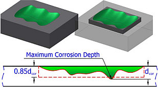
There dcor represents argument depth.

Usage

b31gmodpf(d, wth, smys, depth, l)

Arguments

Details

Since the definition of flow stress, Sflow, in ASME B31G-2012 is recommended with Level 1 as follows:

Sflow = 1.1SMYS

no other possibilities of its evaluation are incorporated.

For this code we avoid possible semantic optimization to preserve readability and correlation with original text description in ASME B31G-2012. At the same time source code for estimated failure pressure preserves maximum affinity with its semantic description in ASME B31G-2012.

Numeric NAs may appear in case prescribed conditions of use are offended.

Value

Estimated failure pressure of the corroded pipe, [PSI]. Type: assert_double.

References

1. ASME B31G-2012. Manual for determining the remaining strength of corroded pipelines: supplement to B31 Code for pressure piping.

2. S. Timashev and A. Bushinskaya, Diagnostics and Reliability of Pipeline Systems, Topics in Safety, Risk, Reliability and Quality 30, DOI 10.1007/978-3-319-25307-7

See Also

Other fail pressure functions: b31gpf, dnvpf, shell92pf, pcorrcpf

Other ASME B31G functions: b31crvl(), b31gacd(), b31gacl(), b31gafr(), b31gdep(), b31gops(), b31gpf(), b31gsap()

Examples

 library(pipenostics)

 ## Example: maximum percentage disparity of original B31G
 ## algorithm and modified B31G showed on CRVL.BAS data
 with(b31gdata, {
   original  <- b31gpf(d, wth, smys, depth, l)
   modified  <- b31gmodpf(d, wth, smys, depth, l)
   round(max(100*abs(1 - original/modified), na.rm = TRUE), 4)
 })
 ## Output:
 #[1] 32.6666

 ## Example: plot disparity of original B31G algorithm and
 ## modified B31G showed on CRVL data
 with(b31gdata[-(6:7),], {
   b31g  <- b31gpf(depth, wth, smys, depth, l)
   b31gmod  <- b31gmodpf(depth, wth, smys, depth, l)
   axe_range <- range(c(b31g, b31gmod))
   plot(b31g, b31g, type = 'b', pch = 16,
        xlab = 'Pressure, [PSI]',
        ylab = 'Pressure, [PSI]',
        main = 'Failure pressure method comparison',
        xlim = axe_range, ylim = axe_range)
   inc <- order(b31g)
   lines(b31g[inc], b31gmod[inc], type = 'b', col = 'red')
   legend('topleft',
          legend = c('B31G Original',
                     'B31G Modified'),
          col = c('black', 'red'),
          lty = 'solid')
 })

ASME B31G. Operational status of pipe

Description

Determine the operational status of pipe: is it excellent? or is technological control required? or is it critical situation?

Usage

b31gops(wth, depth)

Arguments

Value

Operational status of pipe as an integer value:

• 1 - excellent

• 2 - monitoring is recommended

• 3 - alert! replace the pipe immediately!

Type: assert_numeric and assert_subset.

References

ASME B31G-1991. Manual for determining the remaining strength of corroded pipelines. A supplement to ASTME B31 code for pressure piping.

See Also

Other ASME B31G functions: b31crvl(), b31gacd(), b31gacl(), b31gafr(), b31gdep(), b31gmodpf(), b31gpf(), b31gsap()

Examples

 library(pipenostics)

 b31gops(.438, .1)
 # [1] 2  # typical status for the most of pipes

 b31gops(.5, .41)
 # [1] 3  # alert! Corrosion depth is too high! Replace the pipe!

ASME B31G. Failure pressure of the corroded pipe (original)

Description

Calculate failure pressure of the corroded pipe according to Original B31G, Level-1 algorithm listed in ASME B31G-2012.

The next assumption of the corrosion shape is adopted by ASME B31G-2012:

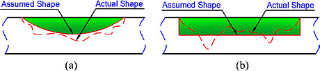
There (a) is a parabolic and (b) is a rectangular idealizations of a corroded area.

Usage

b31gpf(d, wth, smys, depth, l)

Arguments

Details

Since the definition of flow stress, Sflow, in ASME B31G-2012 is recommended with Level 1 as follows:

Sflow = 1.1SMYS

no other possibilities of its evaluation are incorporated.

For this code we avoid possible semantic optimization to preserve readability and correlation with original text description in ASME B31G-2012. At the same time source code for estimated failure pressure preserves maximum affinity with its semantic description in ASME B31G-2012 and slightly differs from that given by Timashev et al. The latter deviates up to 0.7 (b31gdata).

Numeric NAs may appear in case prescribed conditions of use are offended.

Value

Estimated failure pressure of the corroded pipe, [PSI]. Type: assert_double.

References

1. ASME B31G-2012. Manual for determining the remaining strength of corroded pipelines: supplement to B31 Code for pressure piping.

2. S. Timashev and A. Bushinskaya, Diagnostics and Reliability of Pipeline Systems, Topics in Safety, Risk, Reliability and Quality 30, DOI 10.1007/978-3-319-25307-7

See Also

Other fail pressure functions: b31gmodpf, dnvpf, shell92pf, pcorrcpf

Other ASME B31G functions: b31crvl(), b31gacd(), b31gacl(), b31gafr(), b31gdep(), b31gmodpf(), b31gops(), b31gsap()

Examples

 library(pipenostics)

 ## Example: maximum percentage disparity of original B31G
 ## algorithm and modified B31G showed on CRVL.BAS data
 with(b31gdata, {
   original  <- b31gpf(d, wth, smys, depth, l)
   modified  <- b31gmodpf(d, wth, smys, depth, l)
   round(max(100*abs(1 - original/modified), na.rm = TRUE), 4)
 })
 ## Output:
 #[1] 32.6666

 ## Example: plot disparity of original B31G algorithm and
 ## modified B31G showed on CRVL data
 with(b31gdata[-(6:7),], {
   b31g  <- b31gpf(depth, wth, smys, depth, l)
   b31gmod  <- b31gmodpf(depth, wth, smys, depth, l)
   axe_range <- range(c(b31g, b31gmod))
   plot(b31g, b31g, type = 'b', pch = 16,
        xlab = 'Pressure, [PSI]',
        ylab = 'Pressure, [PSI]',
        main = 'Failure pressure method comparison',
        xlim = axe_range, ylim = axe_range)
   inc <- order(b31g)
   lines(b31g[inc], b31gmod[inc], type = 'b', col = 'red')
   legend('topleft',
          legend = c('B31G Original',
                     'B31G Modified'),
          col = c('black', 'red'),
          lty = 'solid')
 })

ASME B31G. Safe maximum pressure for the corroded area of pipe

Description

Calculate safe maximum pressure for the corroded area of pipe.

Usage

b31gsap(dep, d, wth, depth, l)

Arguments

Value

Safe maximum pressure for the corroded area of pipe, [PSI]. Type: assert_double.

References

ASME B31G-1991. Manual for determining the remaining strength of corroded pipelines. A supplement to ASTME B31 code for pressure piping.

See Also

Other ASME B31G functions: b31crvl(), b31gacd(), b31gacl(), b31gafr(), b31gdep(), b31gmodpf(), b31gops(), b31gpf()

Examples

 library(pipenostics)

 b31gsap(1093, 30, .438, .1, 7.5)
 # [1] 1093  # [PSI], safe pressure is equal to design pressure

 b31gsap(877, 24, .281, .08, 15)
 # [1] 690   # [PSI], safe pressure is lower than design pressure due corrosion

Convert to Celsius scale

Description

Convert temperature measured in Kelvin- or Fahrenheit-scale to Celsius (°C).

Usage

c_k(x)

c_f(x)

Arguments

Value

temperature in Celsius-scale, [°C]. Type: assert_double.

See Also

k_c and f_c for converting from Celsius-scale.

Other units: f_k(), inch_mm(), k_c(), kgf_mpa(), loss_flux(), mm_inch(), mpa_kgf(), mpa_psi(), psi_mpa()

Examples

 library(pipenostics)

# Convert from Kelvin to Celsius:
c_k(c(0, 373.15))
# [1]  -273.15  100

# Convert from Fahrenheit to Celsius:
c_f(c(-459.67, 212))
# [1]  -273.15  100

DNV-RP-F101. Failure pressure of the corroded pipe

Description

Calculate failure pressure of the corroded pipe according to Section 8.2 of in DNV-RP-F101. The estimation is valid for single isolated metal loss defects of the corrosion/erosion type and when only internal pressure loading is considered.

The next assumption of the corrosion shape is adopted by DNV-RP-F101:

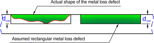
There dcor represents argument depth.

Usage

dnvpf(d, wth, uts, depth, l)

Arguments

Details

In contrast to ASME B31G-2012 property of pipe metal is characterized by specified minimum tensile strength - SMTS, [N/mm^2], and SI is default unit system. SMTS is given in the linepipe steel material specifications (e.g. API 5L) for each material grade.

At the same time Timashev et al. used ultimate tensile strength - UTS in place of SMTS. So, for the case those quantities may be used in interchangeable way.

Numeric NAs may appear in case prescribed conditions of use are offended.

Value

Estimated failure pressure of the corroded pipe, [MPa]. Type: assert_double.

References

1. Recommended practice DNV-RP-F101. Corroded pipelines. DET NORSKE VERITAS, October 2010.

2. ASME B31G-2012. Manual for determining the remaining strength of corroded pipelines: supplement to B31 Code for pressure piping.

3. S. Timashev and A. Bushinskaya, Diagnostics and Reliability of Pipeline Systems, Topics in Safety, Risk, Reliability and Quality 30, DOI 10.1007/978-3-319-25307-7.

See Also

Other fail pressure functions: b31gpf, b31gmodpf, shell92pf, pcorrcpf

Other DNV-RP-F101 functions: strderate()

Examples

 library(pipenostics)

d     <- c(812.8, 219.0)  # [mm]
wth   <- c( 19.1,  14.5)  # [mm]
uts   <- c(530.9, 455.1)  # [N/mm^2]
l     <- c(203.2, 200.0)  # [mm]
depth <- c( 13.4,   9.0)  # [mm]

dnvpf(d, wth, uts, depth, l)
# [1] 15.86626 34.01183

Flow rate drop in pipe

Description

Calculate drop or recovery of flow rate in pipe using geometric factors.

The calculated value may be positive or negative. When it is positive they have the drop, i.e. the decrease of flow rate in the outlet of pipe under consideration. When the calculated value is negative they have the recovery, i.e. the increase of flow rate in the outlet of pipe under consideration. In both cases to calculate flow rate on the outlet of pipe under consideration simply subtract the calculated value from the sensor-measured flow rate on the inlet.

Usage

dropg(adj = 0, d = 700, flow_rate = 250)

Arguments

Details

It is common that sensor-measured flow rate undergoes discharges to network and recharges from it. For calculation of flow rate drop or recovery the next configuration of district heating network segment is assumed:

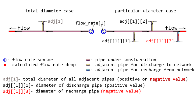
Usually, there are no additional sensors that could measure flow rate in each flow fork. In that case they only may operate with geometric factors, i.e. assuming that flow rate is proportional to square of pipe diameter.

The simple summation of flow rates over all adjacent pipes produces the required flow rate drop or recovery located on the outlet of the pipe under consideration. Since there is concurrency between discharges and recharges the diameters of discharge pipes are regarded positive whereas diameters of recharge pipes must be negative.

Be careful when dealing with geometric factors for large amount of recharges from network: there are no additional physical constraints and thus the calculated value of recovery may have non-sense.

Value

flow rate drop or recovery at the outlet of pipe, [ton/hour], numeric vector. The value is positive for drop, whereas for recovery it is negative. In both cases to calculate flow rate on the outlet of pipe under consideration simply subtract the calculated value from the sensor-measured flow rate on the inlet. Type: assert_double.

See Also

Other district heating: dropp(), dropt()

Examples

 library(pipenostics)

# Let consider pipes according to network segment scheme depicted in figure
# in [?dropg] help-page.

# Typical large diameters of pipes under consideration, [mm]:
d <- as.double(unique(subset(pipenostics::m325nhldata, diameter > 700)$diameter))

# Let sensor-measured flow rate in the inlet of pipe
# under consideration be proportional to d, [ton/hour]:
flow_rate <- .125*d

# Let consider total diameter case when total diameters of adjacent pipes are no
# more than d, [mm]:
adj <- c(450, -400, 950, -255, 1152)

# As at may be seen for the second and fourth cases they predominantly have
# recharges from network.
# Let calculate flow rate on the outlet of the pipe under consideration,
# [ton/hour]

result <- flow_rate - dropg(adj, d, flow_rate)
print(result)

# [1]  75.96439 134.72222  65.70302 180.80580  78.05995

# For more clarity they may perform calculations in `data.table`.

Pressure drop in pipe

Description

Calculate pressure drop in straight cylidrical steel pipe of district heating system (where water is a heat carrier) that is a result of pipe orientation in space (hydrostatic component), and friction between water and internal wall of pipe.

Usage

dropp(
  temperature = 130,
  pressure = mpa_kgf(6),
  flow_rate = 1276,
  d = 1,
  len = 1,
  roughness = 0.006,
  inlet = 0,
  outlet = 0,
  method = "romeo"
)

Arguments

Details

The underlying engineering model for calculation of pressure drop considers only two contributions (components):

1. Pressure drop due to gravity (hydrostatic component).

2. Pressure drop due to friction.

The model does not consider any size changes of pipe and presence of fittings.

For the first component that depends on pipe position in space the next figure illustrates adopted disposition of pipe.

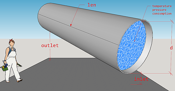
So, the expression for the first component can be written as:

g \rho (outlet - inlet)

where g - is gravity factor, m/s^2, and \rho - density of water (heat carrier), kg/m^3; inlet and outlet are appropriate pipe elevations (under sea or any other adopted level), m.

The second component comes from Darcy–Weisbach equation and is calculated using heating carrier regime parameters (temperature, pressure, flow_rate). Temperature and pressure values of heat carrier define water properties according to IAPWS formulation.

Several methods for calculating of Darcy friction factor are possible and limited to the next direct approximations of Colebrook equation:

romeo

Romeo, Royo and Monzon, 2002

vatankhan

Vatankhan and Kouchakzadeh, 2009

buzelli

Buzzelli, 2008

According to Brkic, 2011 approximations errors of those methods do not exceed 0.15 % for the most combinations of Reynolds numbers and actual values of internal wall roughness of pipe.

Value

pressure drop at the outlet of pipe, [MPa]. Type: assert_double.

References

• W.Wagner et al. The IAPWS Industrial Formulation 1997 for the Thermodynamic Properties of Water and Steam, J. Eng. Gas Turbines Power. Jan 2000, 122(1): 150-184 (35 pages)

• M.L.Huber et al.New International Formulation for the Viscosity of H_2O, Journal of Physical and Chemical Reference Data 38, 101 (2009);

• D.Brkic. Journal of Petroleum Science and Engineering, Vol. 77, Issue 1, April 2011, Pages 34-48.

• Romeo, E., Royo, C., Monzon, A., 2002. Improved explicit equation for estimation of friction factor in rough and smooth pipes. Chem. Eng. J. 86 (3), 369–374.

• Vatankhah, A.R., Kouchakzadeh, S., 2009. Discussion: Exact equations for pipeflow problems, by P.K. Swamee and P.N. Rathie. J. Hydraul. Res. IAHR 47 (7), 537–538.

• Buzzelli, D., 2008. Calculating friction in one step. Mach. Des. 80 (12), 54–55.

See Also

dropt for calculating temperature drop in pipe

Other district heating: dropg(), dropt()

Examples

 library(pipenostics)

# Typical pressure drop for horizontal pipeline segments
# in high-way heating network in Novosibirsk
dropp(len = c(200, 300))

#[1] 0.0007000666 0.0010500999

Temperature drop in cylindrical steel pipe due heat loss

Description

Calculate temperature drop in steel pipe of district heating system (where water is a heat carrier) that is a result of heat loss through pipe wall and insulation.

Usage

dropt(
  temperature = 130,
  pressure = mpa_kgf(6),
  flow_rate = 250,
  loss_power = 7000
)

Arguments

Details

Specific isobaric heat capacity used in calculations is calculated according to IAPWS R7-97(2012) for Region 1 since it is assumed that state of water in district heating system is always in that region.

Value

temperature drop at the outlet of pipe, [°C]. Type: assert_double.

See Also

Other district heating: dropg(), dropp()

Examples

 library(pipenostics)

 # Calculate normative temperature drop based on Minenergo-325 for pipe segment
 pipeline <- list(
   year   = 1968,
   laying = "channel",
   d      = 700, # [mm]
   len    = 1000 # [m]
 )

 regime <- list(
   temperature = c(130, 150), # [°C]
   pressure    = .588399,     # [MPa]
   flow_rate   = 250          # [ton/hour]
 )

 pipe_loss_power <- do.call(
     m325nhl,
     c(pipeline, temperature = list(regime[["temperature"]]), duration = 1)  # [kcal/hour]
 )

 temperature_drop <- dropt(
   temperature = regime[["temperature"]], # [°C]
   loss_power  = pipe_loss_power          # [kcal/hour]
 )                                        # [°C]

 print(temperature_drop)

 # [1] 1.366806 1.433840

Convert to Fahrenheit scale

Description

Convert temperature measured in Kelvin- or Celsius-scale to Fahrenheit (°F).

Usage

f_k(x)

f_c(x)

Arguments

Value

temperature in Fahrenheit-scale, [°F]. Type: assert_double.

See Also

k_f and c_f for converting from Fahrenheit-scale.

Other units: c_k(), inch_mm(), k_c(), kgf_mpa(), loss_flux(), mm_inch(), mpa_kgf(), mpa_psi(), psi_mpa()

Examples

 library(pipenostics)

# Convert from Kelvin to Fahrenheit:
f_k(c(0, 373.15))
# [1]  -459.67 212

# Convert from Celsius to Fahrenheit:
f_c(c(-273.15, 100))
# [1]  -459.67, 212

List all possible flow paths in district heating network

Description

Find and list all possible paths of heat carrier flow (water) in the given topology of district heating system.

Usage

flowls(sender = "A", acceptor = "B", use_cluster = FALSE)

Arguments

Details

Only branched topology without cycles is considered where no more than one incoming edge exists for every acceptor node. For instance, m325testbench has permitted topology.

Though input arguments are natively vectorized their individual values all relate to common part of district heating network, i.e. associated with common object. It is due to isomorphism between vector representation and directed graph of this network. For more details of isomorphic topology description see m325testbench.

Value

named list that contains integer vectors as its elements. The name of each element in the list is the name of acceptor associated with terminal node of district heating network. Each vector in the list represents an ordered sequence of indexes in acceptor that enumerates incoming edges from starting node to terminal one. The length of returned list is equal to number of terminal nodes for topology considered. Type: assert_list.

See Also

m325testbench for example of topology of district heating system

Examples

 library(pipenostics)


# Find path from A to B in trivial line topology:
flowls("A", "B")

# $B
# [1] 1

# More complex example with two terminal nodes D and E:
flowls(c("A", "B", "B"), c("B", "D", "E"))

#$D
#[1] 1 2
#
#$E
#[1] 1 3

# All possible flow paths in test bench illustrated in `?m325testbench`:
all_paths <- list(
  c(12, 13, 11, 8, 4, 1),  # hereinafter indexes of acceptor nodes
  c(12, 13, 11, 8, 4, 2),
  c(12, 13, 11, 8, 6, 5,  3),
  c(12, 13, 11, 8, 6, 7),
  c(12, 13, 11, 8, 6, 9),
  c(12, 13, 11, 10),
  c(12, 13, 14, 15),
  c(12, 13, 16, 17),
  c(12, 13, 16, 18, 20, 19),
  c(12, 13, 16, 18, 20, 21),
  c(12, 13, 16, 18, 22, 24),
  c(12, 13, 16, 18, 22, 25),
  c(12, 13, 16, 18, 20, 23, 26)
)

# find those paths:
path <- with(pipenostics::m325testbench, {
  flowls(sender, acceptor)
})

path[[4]]
# [1] 12 13 11  8  6  7

Estimate pipe friction factor with Buzelli formula

Description

Estimate Darcy friction factor explicitly with extremely accurate Buzelli approximation of Colebrook equation.

Usage

fric_buzelli(reynolds, roughness = 0, strict = FALSE)

Arguments

Details

Buzelli's formula is reported to be extremely accurate in the region:

• 3.0e3 <= reynolds <= 3.0e8

• 0 <= roughness <= 0.05

In strict = TRUE mode argument values outside this precision region are not allowed, whereas in strict = FALSE either NAs are generated in that case or calculation for laminar flow is performed when reynolds < 2100.0.

Value

pipe friction factor, []. Type: assert_double.

References

1. Offor, U. and Alabi, S. (2016) An Accurate and Computationally Efficient Explicit Friction Factor Model. Advances in Chemical Engineering and Science, 6, pp. 237-245. doi:10.4236/aces.2016.63024.

2. Buzzelli, D. (2008) Calculating friction in one step. Machine Design, 80 (12), pp. 54–55.

See Also

Other Fluid properties: fric_romeo(), fric_vatankhan(), re_u()

Examples

 library(pipenostics)

 fric_buzelli(c(2118517, 2000, 2118517), c(1e-6, 70e-3/1, 7e-3/1))
 # [1] 0.01031468 0.03200000 0.03375076  # []

 fric_buzelli(c(2118517, 5500, 2118517), c(1e-6, 50e-3/1, 7e-3/1), TRUE)
 # [1] 0.01031468 0.07556734 0.03375076

Estimate pipe friction factor with Romeo's formula

Description

Estimate Darcy friction factor explicitly with extremely accurate Romeo-Royo-Monzón approximation of Colebrook equation.

Usage

fric_romeo(reynolds, roughness = 0, strict = FALSE)

Arguments

Details

Romeo's formula is reported to be extremely accurate in the region:

• 3.0e3 <= reynolds <= 1.5e8

• 0.0 <= roughness <= 0.05

In strict = TRUE mode argument values outside this precision region are not allowed, whereas in strict = FALSE either NAs are generated in that case or calculation for laminar flow is performed when reynolds < 2100.0.

Value

pipe friction factor, []. Type: assert_double.

References

1. Offor, U. and Alabi, S. (2016) An Accurate and Computationally Efficient Explicit Friction Factor Model. Advances in Chemical Engineering and Science, 6, pp. 237-245. doi:10.4236/aces.2016.63024.

2. Eva Romeo, Carlos Royo, Antonio Monzón, Improved explicit equations for estimation of friction factor in rough and smooth pipes, Chemical Engineering Journal, Volume 86, Issue 3, 2002, Pages 369-374, ISSN 1385-8947. doi:10.1016/S1385-8947(01)00254-6.

See Also

Other Fluid properties: fric_buzelli(), fric_vatankhan(), re_u()

Examples

 library(pipenostics)

 fric_romeo(c(2118517, 2000, 2118517), c(0, 70e-3/1, 7e-3/1))
 # [1] 0.01028473 0.03200000 0.03373215  # []

 fric_romeo(c(2118517, 3030, 2118517), c(0, 50e-3/1, 7e-3/1), TRUE)
 # [1] 0.01028473 0.07859636 0.03373215  # []

Estimate pipe friction factor with Vatankhah formula

Description

Estimate Darcy friction factor explicitly with extremely accurate Vatankhah-Kouchakzadeh approximation of Colebrook equation.

Usage

fric_vatankhan(reynolds, roughness = 0, strict = FALSE)

Arguments

Details

Vatankhah's formula is reported to be extremely accurate in the region:

• 5.0e3 <= reynolds <= 1.0e8

• 1e-6 <= roughness <= 0.05

In strict = TRUE mode argument values outside this precision region are not allowed, whereas in strict = FALSE either NAs are generated in that case or calculation for laminar flow is performed when reynolds < 2100.0.

Value

pipe friction factor, []. Type: assert_double.

References

1. Offor, U. and Alabi, S. (2016) An Accurate and Computationally Efficient Explicit Friction Factor Model. Advances in Chemical Engineering and Science, 6, pp. 237-245. doi:10.4236/aces.2016.63024.

2. Ali R. Vatankhah, Salah Kouchakzadeh (2009) Exact equations for pipe-flow problems. Journal of Hydraulic Research, 47:4, pp. 537-538, DOI: doi:10.1080/00221686.2009.9522031

See Also

Other Fluid properties: fric_buzelli(), fric_romeo(), re_u()

Examples

 library(pipenostics)

 fric_vatankhan(c(2118517, 2000, 2118517), c(1e-6, 70e-3/1, 7e-3/1))
 # [1] 0.01031665 0.03200000 0.03375210  # []

 fric_vatankhan(c(2118517, 5500, 2118517), c(1e-6, 50e-3/1, 7e-3/1), TRUE)
 # [1] 0.01031665 0.07556163 0.03375210

Calculate geographical metrics

Description

Calculate geographical metrics (distance, area) for two or three geographical locations.

Usage

geoarea(lat1, lon1, lat2, lon2, lat3, lon3, earth = 6371008.7714)

geodist(lat1, lon1, lat2, lon2, earth = 6371008.7714)

Arguments

Details

geodist calculates distance between two geographical locations on Earth, whereas geoarea calculates the area of spherical triangle between three geographical locations. Both functions use absolute positions of geographical locations described by geographical coordinate system in decimal degrees units denoted as DD. The haversine formula is applied to calculate the distance, and so the spherical model of Earth is considered in both functions.

Since several variants of Earth radius can be accepted, the user is welcome to provide its own value. WGS-84 mean radius of semi-axes, R_1, is the default value.

The resulting distance is expressed in metres (m), whereas the area is expressed in square kilometers(km^2).

Value

For geodist:

distance between two geographical locations, [m].

For geoarea:

area of spherical triangle between three geographical locations, [km^2].

Type: assert_double.

See Also

Other utils: meteos(), mgtdhid(), wth_d()

Examples

library(pipenostics)

# Consider the longest linear pipeline segment in Krasnoyarsk, [DD]:
pipe <- list(
  lat1 = 55.98320350, lon1 = 92.81257226,
  lat2 = 55.99302417, lon2 = 92.80691885
)

# and some official Earth radii, [m]:
R <- c(
  nominal_zero_tide_equatorial = 6378100.0000,
  nominal_zero_tide_polar      = 6356800.0000,
  equatorial_radius            = 6378137.0000,
  semiminor_axis_b             = 6356752.3141,
  polar_radius_of_curvature    = 6399593.6259,
  mean_radius_R1               = 6371008.7714,
  same_surface_R2              = 6371007.1810,
  same_volume_R3               = 6371000.7900,
  WGS84_ellipsoid_axis_a       = 6378137.0000,
  WGS84_ellipsoid_axis_b       = 6356752.3142,
  WGS84_ellipsoid_curvature_c  = 6399593.6258,
  WGS84_ellipsoid_R1           = 6371008.7714,
  WGS84_ellipsoid_R2           = 6371007.1809,
  WGS84_ellipsoid_R3           = 6371000.7900,
  GRS80_axis_a                 = 6378137.0000,
  GRS80_axis_b                 = 6356752.3141,
  spherical_approx             = 6366707.0195,
  meridional_at_the_equator    = 6335439.0000,
  Chimborazo_maximum           = 6384400.0000,
  Arctic_Ocean_minimum         = 6352800.0000,
  Averaged_center_to_surface   = 6371230.0000
)

# Calculate length of the pipeline segment for different radii:
len <- with(
  pipe, vapply(
    R, geodist, double(1), lat1 = lat1, lon1 = lon1, lat2 = lat2, lon2 = lon2
  )
)

print(range(len))

# [1] 1140.82331483 1152.37564656 #  [m]


# Consider some remarkable objects on Earth, [DD]:
objects <- rbind(
  Mount_Kailash      = c(lat = 31.069831297551982, lon =  81.31215667724196),
  Easter_Island_Moai = c(lat =-27.166873910247862, lon =-109.37092217323053),
  Great_Pyramid      = c(lat = 29.979229451772856, lon =  31.13418110843685),
  Antarctic_Pyramid  = c(lat = -79.97724194984573, lon = -81.96170583068950),
  Stonehendge        = c(lat = 51.179036665131870, lon =-1.8262150017463086)
)

# Consider all combinations of distances between them:
path <- t(combn(rownames(objects), 2))

d <- geodist(
  lat1 = objects[path[, 1], "lat"],
  lon1 = objects[path[, 1], "lon"],
  lat2 = objects[path[, 2], "lat"],
  lon2 = objects[path[, 2], "lon"]
)*1e-3

cat(
  paste(
    sprintf("%s <--- %1.4f km ---> %s", path[, 1], d, path[, 2]),
    collapse = "\n"
)
)

# Consider two areas 
#         * Bermuda triangle     * Polynesian Triangle
lat1 <- c(Miami   =  25.789106,  Hawaii       =   19.820680)
lon1 <- c(Miami   = -80.226529,  Hawaii       = -155.467989)

lat2 <- c(Bermuda =  32.294887,  NewZeland    =  -43.443219)
lon2 <- c(Bermuda = -64.781380,  NewZeland    =  170.271360)

lat3 <- c(SanJuan =  18.466319,  EasterIsland =  -27.112701)
lon3 <- c(SanJuan = -66.105743,  EasterIsland = -109.349668)

# Area provided by manually operated Google Earth:
GETriangleArea <- c(
  Bermuda    =  1147627.48,  # [km^2]
  Polynesian = 28775517.77   # [km^2]
)

# Show the discrepancy in calculations, [km^2]:
print(geoarea(lat1, lon1, lat2, lon2, lat3, lon3)) 
 
 #   Bermuda Polynesian 
 # 0.4673216 11.1030971    

Millimeters to inches

Description

Convert length measured in millimeters (mm) to inches

Usage

inch_mm(x)

Arguments

Value

length in inches, [inch]. Type: assert_double.

See Also

mm_inch for converting inches to mm

Other units: c_k(), f_k(), k_c(), kgf_mpa(), loss_flux(), mm_inch(), mpa_kgf(), mpa_psi(), psi_mpa()

Examples

 library(pipenostics)

 inch_mm(c(25.4, 1))
 # [1] 1.00000000 0.03937008  # [inch]

Covert to Kelvin scale

Description

Convert temperature measured in Celsius- or Fahrenheit-scale to Kelvin (K).

Usage

k_c(x)

k_f(x)

Arguments

Value

temperature in Kelvin-scale, [K]. Type: assert_double.

See Also

c_k and f_k for converting from Kelvin-scale.

Other units: c_k(), f_k(), inch_mm(), kgf_mpa(), loss_flux(), mm_inch(), mpa_kgf(), mpa_psi(), psi_mpa()

Examples

 library(pipenostics)

# Convert from Celsius to Kelvin:
k_c(c(-273.15, 100))
# [1]  0  373.15

# Convert from Fahrenheit to Kelvin:
k_f(c(-459.67, 212))
# [1]  0  373.15

Megapascals to kilogram-force per square

Description

Convert pressure (stress) measured in megapascals (MPa) to kilogram-force per square cm (kgf/cm^2).

Usage

kgf_mpa(x)

Arguments

Value

pressure (stress) in kilogram-force per square cm, [kgf/cm^2]. Type: assert_double.

See Also

mpa_kgf for converting kilogram-force per square cm to megapascals

Other units: c_k(), f_k(), inch_mm(), k_c(), loss_flux(), mm_inch(), mpa_kgf(), mpa_psi(), psi_mpa()

Examples

 library(pipenostics)

 kgf_mpa(c(0.0980665, 1))
 # [1]  1.00000 10.19716

Convert heat flux to specific heat loss power

Description

Convert heat flux measured for a cylindrical steel pipe to specific heat loss power of pipe.

Usage

loss_flux(x, d, wth = 0)

flux_loss(x, d, wth = 0)

Arguments

Value

value of

• specific heat loss power, [kcal/m/h], for loss_flux(x, d, wth)

• heat flux, [W/m^2], for flux_loss(x, d, wth)(x)

Type: assert_double.

See Also

Other units: c_k(), f_k(), inch_mm(), k_c(), kgf_mpa(), mm_inch(), mpa_kgf(), mpa_psi(), psi_mpa()

Examples

library(pipenostics)

# Consider pipes:
diameter      <- c(998, 1395)  # [mm]
wall_thikness <- c(  2,    5)  # [mm]

# Then maximum possible normative neat loss according (Minenergo-325) for
# these pipe diameters are
loss_max <- c(218, 1040)  # [kcal/m/h]

# The appropriate flux is
flux <- flux_loss(loss_max, diameter * 1e-3, wall_thikness)
print(flux)

# [1] 80.70238 275.00155  # [W/m^2]

stopifnot(
  all.equal(loss_flux(flux, diameter * 1e-3, wall_thikness), loss_max, tolerance = 5e-6)
)

Minenergo-278. Normative heat loss of open-air pipe

Description

Calculate normative heat loss of the open-air supplying pipe as a function of construction, operation, and technical condition specifications according to Appendix 5.1 of Minenergo Method 278.

This type of calculations is usually made on design stage of district heating network (where water is a heat carrier) and is closely related to building codes and regulations.

Usage

m278hlair(
  t1 = 110,
  t2 = 60,
  t0 = 5,
  insd1 = 0.1,
  insd2 = insd1,
  d1 = 0.25,
  d2 = d1,
  lambda1 = 0.09,
  lambda2 = 0.07,
  k1 = 1,
  k2 = k1,
  lambda0 = 26,
  len = 1,
  duration = 1
)

Arguments

Details

Details on using k1 and k2 are the same as for m278hlcha.

Value

Normative heat loss of the open-air layed supplying cylindrical pipe during duration, [kcal]. If len of pipe is 1 m (meter) as well as duration is set to 1 h (hour) (default values) then the return value is also the specific heat loss power, [kcal/m/h] and so comparable with those prescribed by Minenergo Order 325. Type: assert_double.

See Also

Other Minenergo: m278hlcha(), m278hlund(), m278insdata, m278inshcm(), m278soildata, m325beta(), m325nhl(), m325nhldata, m325testbench

Examples

 library(pipenostics)

 m278hlair()
 # [1] 138.7736

Minenergo-278. Normative heat loss of pipe in channel

Description

Calculate normative heat loss of the supplying pipe mounted in underground channel as a function of construction, operation, and technical condition specifications according to Appendix 5.1 of Minenergo Method 278.

This type of calculations is usually made on design stage of district heating network (where water is a heat carrier) and is closely related to building codes and regulations.

Usage

m278hlcha(
  t1 = 110,
  t2 = 60,
  t0 = 5,
  insd1 = 0.1,
  insd2 = insd1,
  d1 = 0.25,
  d2 = d1,
  lambda1 = 0.09,
  lambda2 = 0.07,
  k1 = 1,
  k2 = k1,
  lambda0 = 1.74,
  z = 2,
  b = 0.5,
  h = 0.5,
  len = 1,
  duration = 1
)

Arguments

Details

k1 and k2 factor values equal to 1 mean the best technical condition of insulation of appropriate pipes, whereas for poor technical state factor values tends to 5 or more.

Nevertheless, when k1 and k2 both equal to 1 the calculated specific heat loss power [kcal/m/h] is sometimes higher than that listed in Minenergo Order 325. One should consider that situation when choosing method for heat loss calculations.

Value

Normative heat loss of supplying cylindrical pipe mounted in channel during duration, [kcal]. If len of pipe is 1 m (meter) as well as duration is set to 1 h (hour) (default values) then the return value is also the specific heat loss power, [kcal/m/h] and so comparable with those prescribed by Minenergo Order 325. Type: assert_double.

See Also

Other Minenergo: m278hlair(), m278hlund(), m278insdata, m278inshcm(), m278soildata, m325beta(), m325nhl(), m325nhldata, m325testbench

Examples

 library(pipenostics)

 m278hlcha()
 #

 ## Naive way to find out technical state (factors k1 and k2) for pipe
 ## segments constructed in 1980:
   optim(
     par = c(1.5, 1.5),
     fn = function(x) {
     # functional to optimize
       abs(
           m278hlcha(k1 = x[1], k2 = x[2]) -
           m325nhl(year = 1980, laying = "channel", d = 250, temperature = 110)
       )
     },
     method = "L-BFGS-B",
     lower = 1.01, upper = 4.4
   )$par
   # [1] 4.285442 4.323628

Minenergo-278. Normative heat loss of underground pipe

Description

Calculate normative heat loss of the supplying underground pipe as a function of construction, operation, and technical condition specifications according to Appendix 5.1 of Minenergo Method 278.

This type of calculations is usually made on design stage of district heating network (where water is a heat carrier) and is closely related to building codes and regulations.

Usage

m278hlund(
  t1 = 110,
  t2 = 60,
  t0 = 5,
  insd1 = 0.1,
  insd2 = insd1,
  d1 = 0.25,
  d2 = d1,
  lambda1 = 0.09,
  lambda2 = 0.07,
  k1 = 1,
  k2 = k1,
  lambda0 = 1.74,
  z = 2,
  s = 0.55,
  len = 1,
  duration = 1
)

Arguments

Details

Details on using k1 and k2 are the same as for m278hlcha.

Value

Normative heat loss of supplying underground cylindrical pipe during duration, [kcal]. If len of pipe is 1 m (meter) as well as duration is set to 1 h (hour) (default values) then the return value is also the specific heat loss power, [kcal/m/h] and so comparable with those prescribed by Minenergo Order 325. Type: assert_double.

See Also

Other Minenergo: m278hlair(), m278hlcha(), m278insdata, m278inshcm(), m278soildata, m325beta(), m325nhl(), m325nhldata, m325testbench

Examples

 library(pipenostics)

 m278hlund()
 # [1] 102.6226

Minenergo-278. Thermal conductivity terms of pipe insulation materials

Description

Data represent values of terms (intercept and factor) for calculating thermal conductivity of pipe insulation as a linear function of temperature of heat carrier (water). Those values are set for different insulation materials in Appendix 5.3 of Minenergo Method 278 as norms.

Usage

m278insdata

Format

A data frame with 39 rows and 4 variables:

id

Number of insulation material table 5.1 of Appendix 5.3 in Minenergo Method 278. Type: assert_integerish.

material

Designation of insulation material more or less similar to those in table 5.1 of Appendix 5.3 in Minenergo Method 278. Type: assert_character.

lambda

Value for intercept, [mW/m/°C]. Type: assert_integer.

k

Value for factor. Type: assert_integer.

Details

Usually the data is not used directly. Instead use function m278inshcm.

Source

https://docs.cntd.ru/document/1200035568

See Also

Other Minenergo: m278hlair(), m278hlcha(), m278hlund(), m278inshcm(), m278soildata, m325beta(), m325nhl(), m325nhldata, m325testbench

Minenergo-278. Thermal conductivity of pipe insulation materials

Description

Get normative values of thermal conductivity of pipe insulation materials affirmed by Minenergo Method 278 as a function of temperature of heat carrier (water).

Usage

m278inshcm(temperature = 110, material = "aerocrete")

Arguments

Value

Thermal conductivity of insulation materials at given set of temperatures, [W/m/°C], [W/m/K]. Type: assert_double.

See Also

Other Minenergo: m278hlair(), m278hlcha(), m278hlund(), m278insdata, m278soildata, m325beta(), m325nhl(), m325nhldata, m325testbench

Examples

 library(pipenostics)

# Averaged thermal conductivity of pipe insulation at 110 °C
print(m278insdata)
mean(m278inshcm(110, m278insdata[["material"]]))
# [1] 0.09033974  # [\emph{W/m/°C}]

Minenergo-278. Thermal conductivity of subsoil surrounding pipe

Description

Data represent normative values of thermal conductivity of subsoils which can surround pipes according to Table 5.3 of Appendix 5.3 in Minenergo Method 278.

Usage

m278soildata

Format

A data frame with 15 rows and 3 variables:

subsoil

Geological name of subsoil. Type: assert_character.

state

The degree of water penetration to the subsoil. Type: assert_character.

lambda

Value of thermal conductivity of subsoil regarding water penetration, [W/m/°C]. Type: assert_double.

Source

https://docs.cntd.ru/document/1200035568

See Also

Other Minenergo: m278hlair(), m278hlcha(), m278hlund(), m278insdata, m278inshcm(), m325beta(), m325nhl(), m325nhldata, m325testbench

Minenergo-325. Local heat loss coefficient

Description

Calculate \beta - local heat loss coefficient according to rule 11.3.3 of Minenergo Order 325. Local heat loss coefficient is used to increase normative heat loss of pipe by taking into account heat loss of fittings (shut-off valves, compensators and supports). This coefficient is applied mostly as a factor during the summation of heat losses of pipes in pipeline leveraging formula 14 of Minenergo Order 325.

Usage

m325beta(laying = "channel", d = 700)

Arguments

Value

Two possible values of \beta: 1.2 or 1.15 depending on pipe laying and its diameter. Type: assert_double.

See Also

Other Minenergo: m278hlair(), m278hlcha(), m278hlund(), m278insdata, m278inshcm(), m278soildata, m325nhl(), m325nhldata, m325testbench

Examples

 library(pipenostics)

norms <- within(m325nhldata, {
  beta <- m325beta(laying, as.double(diameter))
})
unique(norms$beta)
# [1] 1.15 1.20

Minenergo-325. Normative heat loss of pipe

Description

Calculate normative heat loss of pipe that is legally affirmed by Minenergo Order 325.

Usage

m325nhl(
  year = 1986,
  laying = "underground",
  exp5k = TRUE,
  insulation = 0,
  d = 700,
  temperature = 110,
  len = 1,
  duration = 1,
  beta = FALSE,
  extra = 2
)

Arguments

Details

Temperature extrapolation and pipe diameter interpolation are leveraged for better accuracy. Both are linear as it dictated by Minenergo Order 325. Nevertheless, one could control the extrapolation behavior by extra argument: use lower values of extra for soft curvature near extrapolation edges, and higher values for more physically reasoned behavior in far regions of extrapolation.

Value

Normative heat loss of cylindrical pipe during duration, [kcal]. If len of pipe is 1 m (meter) as well as duration is set to 1 h (hour) (default values) then the return value is also the specific heat loss power, [kcal/m/h], prescribed by Minenergo Order 325. Type: assert_double.

See Also

Other Minenergo: m278hlair(), m278hlcha(), m278hlund(), m278insdata, m278inshcm(), m278soildata, m325beta(), m325nhldata, m325testbench

Examples

 library(pipenostics)

 ## Consider a 1-meter length pipe with
 pipe_diameter <-  700.0  # [mm]
 pipe_dating   <- 1980
 pipe_laying   <- "underground"


 ## Linear extrapolation adopted in Minenergo's Order 325 using last two points:
 operation_temperature <- seq(0, 270, 10)

 qs <- m325nhl(
   year = pipe_dating, laying = pipe_laying, d = pipe_diameter,
   temperature = operation_temperature
 )  # [kcal/m/h]

 plot(
     operation_temperature,
     qs,
     type = "b",
     main = "Minenergo's Order 325. Normative heat loss of pipe",
     sub = sprintf(
       "%s pipe of diameter %i [mm] laid in %i",
        pipe_laying, pipe_diameter, pipe_dating
     ),
     xlab = "Temperature, [°C]",
     ylab = "Specific heat loss power, [kcal/m/h]"
   )


 ## Consider heat loss due fittings:
 operation_temperature <- 65  # [°C]

 fittings_qs <- m325nhl(
   year = pipe_dating, laying = pipe_laying, d = pipe_diameter,
   temperature = operation_temperature, beta = c(FALSE, TRUE)
 )  # [kcal/m/h]

 print(fittings_qs); stopifnot(all(round(fittings_qs ,1)  == c(272.0, 312.8)))

 # [1] 272.0 312.8  # [kcal/m/h]



 ## Calculate heat flux:
 operation_temperature <- c(65, 105)  # [°C]

 qs <- m325nhl(
   year = pipe_dating, laying = pipe_laying, d = pipe_diameter,
   temperature = operation_temperature
 )  # [kcal/m/h]
 print(qs)

 # [1] 272.00 321.75  # [kcal/m/h]

 pipe_diameter <- pipe_diameter * 1e-3          # [m]
 factor        <- 2.701283                      # [kcal/h/W]

 flux <- qs/factor/pipe_diameter -> a  # heat flux, [W/m^2]
 print(flux)

 # [1] 143.8470 170.1572  # [W/m^2]

 ## The above line is equivalent to:

 flux <- flux_loss(qs, pipe_diameter) -> b

 stopifnot(all.equal(a, b, tolerance = 5e-6))

Minenergo-325. Normative heat loss data

Description

Data represent values of specific heat loss power officially accepted by Minenergo Order 325 as norms. Those values are maximums which are legally affirmed to contribute to normative heat loss Q_NHL of district heating systems with water as a heat carrier.

Usage

m325nhldata

Format

A data frame with 17328 rows and 8 variables:

source

Identifier of data source: identifiers suited with glob t?p? mean appropriate table ?.? in Minenergo Order 325; identifier sgc means that values are additionally postulated (see Details). Type: assert_character.

epoch

Year depicting the epoch when the pipe is put in operation after laying or total overhaul. Type: assert_integer.

laying

Type of pipe laying depicting the position of pipe in space. Only five types of pipe laying are considered:

• air,

• channel,

• room,

• tunnel,

• underground.

Type: assert_character.

exp5k

Logical indicator for pipe regime: if TRUE pipe is operated more that 5000 hours per year. Type: assert_logical.

insulation

Identifier of insulation that covers the exterior of pipe:

0

no insulation

1

foamed polyurethane or analogue

2

polymer concrete

Type: assert_integerish.

diameter

Nominal internal diameter of pipe, [mm]. Type: assert_double.

temperature

Operational temperature of pipe, [°C]. Type: assert_double.

loss

Normative value of specific heat loss power equal to heat flux output by 1 meter length steel pipe during an hour, [kcal/m/hour]. Type: assert_double.

Details

Data is organized as a full factorial design, whereas for some factorial combinations Minenergo Order 325 does not provide values. For that cases values are postulated by practical reasons in Siberian cities and marked with source label sgc.

Usually the data is not used directly. Instead use function m325nhl.

Source

https://docs.cntd.ru/document/902148459

See Also

Other Minenergo: m278hlair(), m278hlcha(), m278hlund(), m278insdata, m278inshcm(), m278soildata, m325beta(), m325nhl(), m325testbench

Minenergo-325. Test bench of district heating network

Description

Data describes a virtual test bench of branched district heating network by exposing parameters associated with Minenergo Order 325. They treat data as a snapshot of network state and use it primarily for static thermal-hydraulic computations and topology effects.

Usage

m325testbench

Format

A data frame with 22 rows (number of nodes and incoming edges) and 15 variables:

sender

An identifier of node which heat carrier flows out. Type: any type that can be painlessly coerced to character by as.character.

acceptor

An identifier of node which heat carrier flows in. According to topology of test bench considered this identifier should be unique for every row. Type: any type that can be painlessly coerced to character by as.character.

temperature

Snapshot of thermal-hydraulic regime state: temperature of heat carrier (water) sensor-measured on terminal acceptor node, [°C]. Type: assert_double. NAs are introduced for nodes without temperature sensor.

pressure

Snapshot of thermal-hydraulic regime state: sensor-measured absolute pressure of heat carrier (water) inside the pipe (i.e. acceptor's incoming edge), [MPa]. Type: assert_double. NAs are introduced for nodes without pressure sensor.

flow_rate

Snapshot of thermal-hydraulic regime state: sensor-measured amount of heat carrier (water) on terminal node that is transferred by pipe (i.e. acceptor's incoming edge) during a period, [ton/hour]. Type: assert_double. NAs are introduced for nodes without flow rate sensor.

d

internal diameter of pipe (i.e.diameter of acceptor's incoming edge), [m]. Type: assert_double.

len

pipe length (i.e. length of acceptor's incoming edge), [m]. Type: assert_double.

year

year when the pipe (i.e. acceptor's incoming edge) is put in operation after laying or total overhaul. Type: assert_integerish.

insulation

identifier of insulation that covers the exterior of pipe (i.e. acceptor's incoming edge):

0

no insulation

1

foamed polyurethane or analogue

2

polymer concrete

Type: assert_integerish.

laying

type of pipe laying depicting the position of pipe in space. Only five types of pipe laying are considered:

• air,

• channel,

• room,

• tunnel,

• underground.

Type: assert_character.

beta

logical indicator: should they consider additional heat loss of fittings located on this pipe (i.e. acceptor's incoming edge)? Type: assert_logical.

exp5k

logical indicator for regime of pipe (i.e. acceptor's incoming edge): if TRUE pipe is operated more that 5000 hours per year. Type: assert_logical.

roughness

roughness of internal wall of pipe (i.e. acceptor's incoming edge), [m]. Type: assert_double.

inlet

elevation of pipe inlet, [m]. Type: assert_double.

outlet

elevation of pipe outlet, [m]. Type: assert_double.

Details

The test bench has the next configuration:

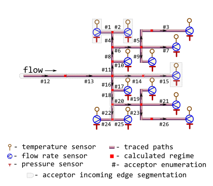
As it may be seen from the figure there is a particularity in topology of the provided directed graph: each node has only single ancestor. Hence one of isomorphic representation of such directed graph is a data.frame in which each row describes a node along with its incoming edge and each column contains an attribute value for that node or an attribute value for its incoming edge.

Since they deal with incoming edges and hence nodes are all flow acceptors the natural enumeration of nodes is by acceptor id.

Note that to leverage igraph functionality for plotting there is a zero sender of flow.

See Also

Other Minenergo: m278hlair(), m278hlcha(), m278hlund(), m278insdata, m278inshcm(), m278soildata, m325beta(), m325nhl(), m325nhldata

Examples

 library(pipenostics)

# Do not hesitate to use `data.table` and `igraph` for larger chunks of network.

# Check for declared topology isomorphism:
stopifnot(
  all(!duplicated(m325testbench$acceptor))
)

# Do all terminal nodes have sensor-measured regime parameters?:
terminal_nodes <- subset(m325testbench, !(acceptor %in% sender))
stopifnot(
  all(!is.na(subset(terminal_nodes, select = c(temperature, pressure, flow_rate))))
)

Minenergo-325. Massively trace backwards thermal-hydraulic regime for district heating network

Description

Trace values of thermal-hydraulic regime (temperature, pressure, flow rate, and other) in the bunched pipeline against the flow direction using norms of heat loss values prescribed by Minenergo Order 325.

Algorithm also suits for partially measurable district heating network with massive data lack conditions, when there are no temperature and pressure sensor readings on the majority of terminal nodes.

Usage

m325tracebw(
  sender = 6,
  acceptor = 7,
  temperature = 70,
  pressure = pipenostics::mpa_kgf(6),
  flow_rate = 20,
  d = 100,
  len = 72.446,
  year = 1986,
  insulation = 0,
  laying = "tunnel",
  beta = FALSE,
  exp5k = TRUE,
  roughness = 0.001,
  inlet = 0.5,
  outlet = 1,
  method = "romeo",
  opinion = "median",
  verbose = TRUE,
  csv = FALSE,
  file = "m325tracebw.csv"
)

Arguments

Details

They consider the topology of district heating network represented by m325testbench:

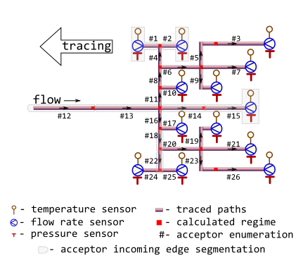
The network may be partially sensor-equipped too:

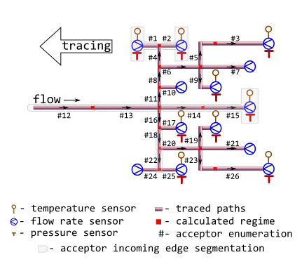
In latter case no more than two nodes must be equipped with pressure and temperature sensors whereas for other nodes only flow rate sensors must be installed.

Tracing starts from sensor-equipped nodes and goes backwards, i.e against the flow direction.

Though some input arguments are natively vectorized their individual values all relate to common part of district heating network, i.e. associated with common object. It is due to isomorphism between vector representation and directed graph of this network. For more details of isomorphic topology description see m325testbench.

Before tracing starts for the next node, previously calculated values of thermal-hydraulic parameters are aggregated by either averaging or by median. The latter seems more robust for avoiding strong influence of possible outliers which may come from actual heating transfer anomalies, erroneous sensor readings or wrong pipeline specifications.

Aggregation for values of flow rate at the node is always sum.

Value

data.frame containing results (detailed log) of tracing in narrow format:

node

Tracing job. Identifier of the node which regime parameters is calculated for. Values in this vector are identical to those in argument acceptor. Type: assert_character.

tracing

Tracing job. Identifiers of nodes from which regime parameters are traced for the given node. Identifier sensor is used when values of regime parameters for the node are sensor readings. Type: assert_character.

backward

Tracing job. Identifier of tracing direction. It constantly equals to TRUE. Type: assert_logical.

aggregation

Tracing job. Identifier of aggregation method: span, median, mean, or identity. Type: assert_character.

loss

Traced thermal hydraulic regime. Normative specific heat loss power of adjacent pipe, [kcal/m/h]. Type: assert_double.

flux

Traced thermal hydraulic regime. Normative heat flux of adjacent pipe, [W/m^2]. Type: assert_double.

Q

Traced thermal hydraulic regime. Normative heat loss of adjacent pipe per day, [kcal]. Type: assert_character.

temperature

Traced thermal hydraulic regime. Traced temperature of heat carrier (water) that is associated with the node, [°C]. Type: assert_double.

pressure

Traced thermal hydraulic regime. Traced pressure of heat carrier (water) that is associated with the node, [MPa]. Type: assert_double.

flow_rate

Traced thermal hydraulic regime. Traced flow rate of heat carrier (water) that is associated with the node, [ton/hour]. Type: assert_double.

job

Tracing job. Value of tracing job counter. Type: assert_count.

Type: assert_data_frame.

See Also

Other Regime tracing: m325tracefw(), m325traceline(), tracebw(), tracefw(), traceline()

Examples

library(pipenostics)

## It is possible to run without specification of argument values:
m325tracebw()

## Consider isomorphic representation of District Heating Network graph:
DHN <- pipenostics::m325testbench
DHN$d <- 1e3*DHN$d  # convert [m] to [mm]

## When tracing large network graphs put screen log to file
output <- do.call("m325tracebw", c(as.list(DHN), verbose = TRUE))

## Distinct options for opinion aggregation lead to distinct traced
## temperature and pressure:

## * When aggregation is by mean:
output_mean <- do.call(
  "m325tracebw", c(as.list(DHN), verbose = FALSE, opinion = "mean")
)

## * When aggregation is by median:
output_median <- do.call(
  "m325tracebw", c(as.list(DHN), verbose = FALSE, opinion = "median")
)

## The differences between aggregations should be:
aggregation_differences <- c(delta_t = 0.03732, delta_p = 0.00139, delta_g = 0)
print(aggregation_differences)

## Check:
stopifnot(
  round(
    subset(
      output_mean,
      node == 13 & aggregation == "median",
      c("temperature", "pressure", "flow_rate")
    ) - subset(
      output_median,
      node == 13 & aggregation == "median",
      c("temperature", "pressure", "flow_rate")
    ),
    5
    # difference between aggregation options
  ) == aggregation_differences
)

## It is possible to process partially measurable District Heating Network:

## * Simulate lack of temperature and pressure sensors:
DHN[c(7, 10, 21, 24), c("temperature", "pressure")] <- NA_real_

## Trace thermal-hydraulic regime
output <- do.call("m325tracebw", c(as.list(DHN)))
print(output)

Minenergo-325. Massively trace forwards thermal-hydraulic regime for district heating network

Description

Trace values of thermal-hydraulic regime (temperature, pressure, flow rate, and other) in the bunched pipeline along the flow direction using norms of heat loss values prescribed by Minenergo Order 325.

Usage

m325tracefw(
  sender = c(0, 1),
  acceptor = c(1, 2),
  temperature = c(70, NA_real_),
  pressure = c(pipenostics::mpa_kgf(6), NA_real_),
  flow_rate = c(20, NA_real_),
  d = rep_len(100, 2),
  len = rep_len(72.446, 2),
  year = rep_len(1986, 2),
  insulation = rep_len(0, 2),
  laying = rep_len("tunnel", 2),
  beta = rep_len(FALSE, 2),
  exp5k = rep_len(TRUE, 2),
  roughness = rep_len(0.001, 2),
  inlet = c(0.5, 1),
  outlet = c(1, 1),
  elev_tol = 0.1,
  method = "romeo",
  verbose = TRUE,
  csv = FALSE,
  file = "m325tracefw.csv",
  use_cluster = FALSE
)

Arguments

Details

The calculated (values of) regime may be considered as representation of district heating process in conditions of hypothetically perfect technical state of pipe walls and insulation.

They consider the topology of district heating network represented by m325testbench:

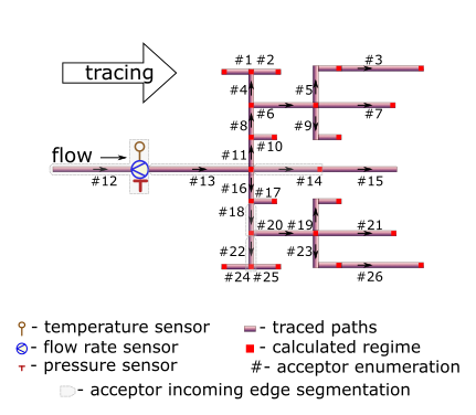
Tracing starts from sensor-equipped root node and goes forward, i.e along the flow direction. Function m325traceline serves under the hood for tracing identified linear segments from root node to every terminal node. Hence they only need root node to be equipped with sensors. Sensors at other nodes are redundant in forward tracing, since the tracing algorithm by no means consider them for tracing.

Moreover in the forward tracing algorithm they assume the flow of heat carrier is distributed proportionally to the cross-sectional area of the outgoing pipeline. Actually, a lot of reasons may cause significant deviations from this assumption. As a result, the sequence of paired backward/forward tracing may be divergent for regime parameters.

Though some input arguments are natively vectorized their individual values all relate to common part of district heating network, i.e. associated with common object. It is due to isomorphism between vector representation and directed graph of this network. For more details of isomorphic topology description see m325testbench.

They are welcome to couple the algorithm with functionality of data.table.

Value

data.frame containing results (detailed log) of tracing in narrow format:

node

Tracing job. Identifier of the node which regime parameters is calculated for. Values in this vector are identical to those in argument acceptor. Type: assert_character.

tracing

Tracing job. Identifiers of nodes from which regime parameters are traced for the given node. Identifier sensor is used when values of regime parameters for the node are sensor readings. Type: assert_character.

backward

Tracing job. Identifier of tracing direction. It constantly equals to FALSE. Type: assert_logical.

aggregation

Tracing job. Identifier of the aggregation method associated with traced values. For forward tracing the only option is identity. Type: assert_character.

temperature

Traced thermal hydraulic regime. Traced temperature of heat carrier (water) that is associated with the node, [°C]. Type: assert_double.

pressure

Traced thermal hydraulic regime. Traced pressure of heat carrier (water) that is associated with the node, [MPa]. Type: assert_double.

flow_rate

Traced thermal hydraulic regime. Traced flow rate of heat carrier (water) that is associated with the node, [ton/hour]. Type: assert_double.

job

Tracing job. Value of tracing job counter. For forward tracing value of job counts the number of traced paths from root node. Type: assert_count.

Type: assert_data_frame.

See Also

Other Regime tracing: m325tracebw(), m325traceline(), tracebw(), tracefw(), traceline()

Examples

library(pipenostics)

# Minimum two nodes should be in district heating network graph:
m325tracefw(verbose = FALSE)

# Consider isomorphic representation of District Heating Network graph:
DHN <- pipenostics::m325testbench

# * avoid using numeric identifiers for nodes:
DHN$sender   <- sprintf("N%02i", DHN$sender)
DHN$acceptor <- sprintf("N%02i", DHN$acceptor)

# * alter units:
DHN$d <- 1e3 * DHN$d  # convert [m] to [mm]

# Perform backward tracing to get regime on root node:
bw_report <- do.call("m325tracebw", c(as.list(DHN), verbose = FALSE))

# Put the traced values to the root node of test bench:
root_node_idx <- 12
root_node <- sprintf("N%02i", root_node_idx)
regime_param  <- c("temperature", "pressure", "flow_rate")
DHN[root_node_idx, regime_param] <-
  subset(bw_report,
         node == root_node & aggregation == "median",
         regime_param)
rm(root_node, root_node_idx)

# Trace the test bench forward for the first time:
fw_report <- do.call("m325tracefw",
                     c(as.list(DHN), verbose = FALSE, elev_tol = .5))

# Let's compare traced regime at terminal nodes back to test bench:
report <- subset(
  rbind(bw_report, fw_report),
  node %in% subset(DHN, !(acceptor %in% sender))$acceptor &
    aggregation == "identity"
)

regime_delta <- colMeans(
  subset(report, backward, regime_param) -
    subset(report, !backward, regime_param)
)
print(regime_delta)

stopifnot(sqrt(regime_delta %*% regime_delta) < 0.5)

Minenergo-325. Trace thermal-hydraulic regime for linear segment of district heating network

Description

Trace values of thermal-hydraulic regime (temperature, pressure, flow_rate, and other) along the adjacent linear segments of pipeline using norms of heat loss values prescribed by Minenergo Order 325.

Usage

m325traceline(
  temperature = 130,
  pressure = mpa_kgf(6),
  flow_rate = 250,
  g = 0,
  d = 700,
  len = c(600, 530, 300, 350),
  year = 1986,
  insulation = 0,
  laying = "underground",
  beta = FALSE,
  exp5k = TRUE,
  roughness = 0.006,
  inlet = 0,
  outlet = 0,
  elev_tol = 0.1,
  method = "romeo",
  forward = TRUE,
  absg = TRUE
)

Arguments

Details

The calculated (values of) regime may be considered as representation of district heating process in conditions of hypothetically perfect technical state of pipe walls and insulation.

They consider only simple tracing paths which do not contain rings and any kind of parallelization. At the same time bidirectional (forward and backward) tracing is possible in accordance with sensor position. They also may consider discharges to network at the inlet of each pipeline segment as an approximation of actual forks of flows. Relevant illustration of adopted assumptions for 4-segment tracing path is depicted on the next figure.

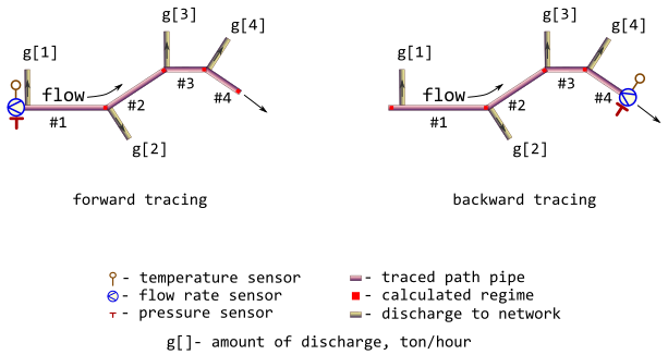
They make additional check for consistency of inlet and outlet values for subsequent pipe segments. Discrepancy of appropriate elevations cannot be more than elev_tol.

Since inner diameter of the pipe is used as input, the the thickness of the pipe wall additionally considered in heat flux calculations. Pipe wall thickness is derived from pipe diameter using GOST 30732 specifications.

Value

list containing results (detailed log) of tracing for each pipe in tracing path enumerated along the direction of flow:

temperature

Traced thermal hydraulic regime. Traced temperature of heat carrier (water), [°C]. Type: assert_double.

pressure

Traced thermal hydraulic regime. Traced pressure of heat carrier (water) for each pipe in tracing path enumerated along the direction of flow, [MPa]. Type: assert_double.

flow_rate

Traced thermal hydraulic regime. Traced flow rate of heat carrier (water) for each pipe in tracing path enumerated along the direction of flow, [ton/hour]. Type: assert_double.

loss

Traced thermal hydraulic regime. Normative specific heat loss power for each pipe in tracing path enumerated along the direction of flow, [kcal/m/h]. Type: assert_double.

flux

Traced thermal hydraulic regime. Normative heat flux for each pipe in tracing path enumerated along the direction of flow, [W/m^2]. Type: assert_double.

Q

Traced thermal hydraulic regime. Normative heat loss for each pipe in tracing path enumerated along the direction of flow per day, [kcal]. Type: assert_double.

Type: assert_list.

See Also

Other Regime tracing: m325tracebw(), m325tracefw(), tracebw(), tracefw(), traceline()

Examples

 library(pipenostics)

# Consider 4-segment tracing path depicted in ?m325regtrace help page.
# First, let sensor readings for forward tracing:
t_fw <- 130  # [°C]
p_fw <- mpa_kgf(6)*all.equal(.588399, mpa_kgf(6))  # [MPa]
g_fw <- 250  # [ton/hour]

# Let discharges to network for each pipeline segment are somehow determined as
discharges <- seq(0, 30, 10)  # [ton/hour]

# Then the calculated regime (red squares) for forward tracing is
regime_fw <- m325traceline(t_fw, p_fw, g_fw, discharges, forward = TRUE)
print(regime_fw)

# $temperature
# [1] 129.1799 128.4269 127.9628 127.3367
#
# $pressure
# [1] 0.5878607 0.5874226 0.5872143 0.5870330
#
# $flow_rate
# [1] 250 240 220 190
#
# $loss
# [1] 348.0000 347.1389 346.3483 345.8610
#
# $flux
# [1] 181.9600 181.5097 181.0963 180.8415
#
# $Q
# [1] 5011200 4415607 2493707 2905232


# Next consider values of traced regime as sensor readings for backward tracing:
t_bw <- 127.3367  # [°C]
p_bw <- .5870330  # [MPa]
g_bw <- 190  # [ton/hour]

# Then the calculated regime (red squares) for backward tracing is
regime_bw <- m325traceline(t_bw, p_bw, g_bw, discharges, forward = FALSE)
print(regime_bw)

# $temperature
# [1] 129.9953 129.1769 128.4254 127.9619
#
# $pressure
# [1] 0.5883998 0.5878611 0.5874228 0.5872144
#
# $flow_rate
# [1] 250 250 240 220
#
# $loss
# [1] 347.1358 346.3467 345.8599 345.2035
#
# $flux
# [1] 181.5081 181.0955 180.8410 180.4978
#
# $Q
# [1] 4998755 4405529 2490192 2899710

# Let compare sensor readings with backward tracing results:
tracing <- with(regime_bw, {
  lambda <- function(val, constraint)
    c(val, constraint, constraint - val,
      abs(constraint - val)*100/constraint)
  first <- 1
  structure(
    rbind(
      lambda(temperature[first], t_fw),
      lambda(pressure[first],    p_fw),
      lambda(flow_rate[first], g_fw)
    ),
    dimnames = list(
      c("temperature", "pressure", "flow_rate"),
      c("sensor.value", "traced.value", "abs.discr", "rel.discr")
    )
  )
})
print(tracing)

# sensor.value traced.value     abs.discr    rel.discr
# temperature  129.9952943   130.000000  4.705723e-03 0.0036197868
# pressure       0.5883998     0.588399 -8.215938e-07 0.0001396321
# flow_rate    250.0000000   250.000000  0.000000e+00 0.0000000000

Probability of failure of the corroded pipe within maximum entropy

Description

Calculate probability of failure (POF) of the corroded pipe taking into account its actual level of defectiveness and exploiting Monte-Carlo simulation within Principle of maximum entropy.

Consistent estimate of POF for pipeline systems plays a critical role in optimizing their operation. To prevent pipeline failures due to actively growing defects it is necessary to be able to assess the pipeline system failure operation probability during a certain period, taking into account its actual level of defectiveness. The pipeline limit state comes when the burst pressure, considered as a random variable, reaches an unacceptable level, or when the defect depth, also a random variable, exceeds the predetermined limit value.

That is why in the method they consider two possible failures for a single pipeline cross section with the on-surface and longitudinally oriented defect of metal-loss type:

rupture

a decrease of value of failure pressure down to the operating pressure.

leak

increase of corrosion depth (defect) up to the specified ultimate permissible fraction of pipe wall thickness.

Since up to now no methods existed which would give absolutely correct POF assessments they suggest simple fiddling with random values of affecting factors without deeping into intrinsic mechanisms of corrossion. For this purpose they choose classical Monte-Carlo simulation within the Principle of maximum entropy. The latter allows to avoid doubtful and excessive preferences and detalization when choosing probability distribution models for failure factors and for inline inspection measurements.

Usage

mepof(
  depth = seq(0, 10, length.out = 100),
  l = seq(40, 50, length.out = 100),
  d = rep.int(762, 100),
  wth = rep.int(10, 100),
  strength = rep.int(358.5274, 100),
  pressure = rep.int(0.588, 100),
  temperature = rep.int(150, 100),
  rar = function(n) stats::runif(n, 0.01, 0.3)/365,
  ral = function(n) stats::runif(n, 0.01, 0.3)/365,
  days = 0,
  k = 0.8,
  method = "b31g",
  n = 1e+06
)

Arguments

Details

Since for all influence factors they can more or less assume range limits, the uniform distribution gets the maximum entropy in this context (see JCGM 101:2008). That is why parameters of corrosion defects measured during the inline inspection as well as regime parameters and engineering characteristics of pipe segment - all they are simulated by runif.

runif-limits for depth of corrosion defect are associated with precision of commonly applied measurement instruments. For traditionally exploited ultrasonic control those limits are well-known and can reach up to 10 % of pipe wall thickness. Whereas uncertainty of defect longitudinal length may be more than enough constrained with 5 %.

Recommendations for choosing stochastic characteristics of pipe engineering factors (i.e. crossection diameter, wall thickness and material strength) are taken from aggregated review of Timashev et al. but gently transformed for compatibility with Principle of maximum entropy, i.e. runif.

Uncertainties of regime parameters in stohastic models are set minimized by regarding only precision of metering devices which commonly applied in district heating networks. For temperature it is about 2 °C.

Since the rate of corrosion processes in the pipe wall is a consequence of physical and chemical processes occurring at the atomic scale, it depends on a large number of environmental factors differently and ambiguously. That is why various deterministic and stochastic models can be potentially involved in POF assessment. For that purpose radial and longitudinal corrosion rate can be independently formulated as random value generation functions. They only admit that change in depth and length of corrosion defects in time is close to linear for the generated value of corrosion rate.

Value

Probability of pipe failure for each corroded area measured during inline inspection. Type: assert_double. If NAs returned use another method for calculating failure pressure.

References

1. S. Timashev and A. Bushinskaya, Diagnostics and Reliability of Pipeline Systems, Topics in Safety, Risk, Reliability and Quality 30, DOI 10.1007/978-3-319-25307-7.

2. BIPM. Guides in Metrology (GUM). JCGM 101:2008. Evaluation of measurement data – Supplement 1 to the Guide to the expression of uncertainty in measurement – Propagation of distributions using a Monte Carlo method.

Examples

 library(pipenostics)


# Let's consider a pipe in district heating network with
diameter           <- 762         # [mm]
wall_thickness     <-  10         # [mm]
UTS                <- 434.3697    # [MPa]

# which transfers heat-carrier (water) at
operating_pressure <-   0.588399  # [MPa].
temperature        <-  95         # [°C]

# During inline inspection four corroded areas (defects) are detected with:
depth  <- c(2.45,  7.86,   7.93,   8.15)  # [mm]

# whereas the length of all defects is not greater 200 mm:
length <- rep(200, 4)  # [mm]

# Corrosion rates in radial and in longitudinal directions are not well-known and
# may vary in range .01 - .30 mm/year:
rar = function(n) stats::runif(n, .01, .30) / 365
ral = function(n) stats::runif(n, .01, .30) / 365

# Then POFs related to each corroded area are near:
pof <- mepof(depth, length, rep(diameter, 4), rep(wall_thickness, 4),
             rep(UTS, 4), rep(operating_pressure, 4), rep(temperature, 4),
             rar, ral, method = "dnv")
print(pof)
# 0.000000 0.252510 0.368275 0.771595

# So, the POF of pipe is near
print(max(pof))
# 0.771595

# The value of POF changes in time. So, in a year after inline inspection of
# the pipe we can get something near
pof <- mepof(depth, length, rep(diameter, 4), rep(wall_thickness, 4),
             rep(UTS, 4), rep(operating_pressure, 4), rep(temperature, 4),
             rar, ral, method = "dnv", days = 365)
print(pof)
# 0.000000 0.525539 0.648359 0.929099

# for entire pipe we get something near:
print(max(pof))
# 0.929099

# Two years ago before inline inspection the pipe state was rather good:
pof <- mepof(depth, length, rep(diameter, 4), rep(wall_thickness, 4),
             rep(UTS, 4), rep(operating_pressure, 4), rep(temperature, 4),
             rar, ral, method = "dnv", days = -2 * 365)

print(pof)
# 0.000000 0.040780 0.072923 0.271751

# for entire pipe we get something near:
print(max(pof))
# 0.271751

Get list of weather stations (meteos)

Description

Get a list of weather stations located primarily in the central and northern parts of Eurasia. For each weather station, the following information is provided: an integer station ID, geographic coordinates, altitude, and the mean annual ground temperature averaged over depth.

Usage

meteos()

Value

list of weather stations (meteos) with the next fields:

station_id

Weather station unique identifier. Type: assert_integer.

name

Human-readable name of weather station. Type: assert_character.

lat

Geographical position of wether station. Latitude, [DD]. Type: assert_double.

lon

Geographical position of wether station. Longitude, [DD]. Type: assert_double.

alt

Altitude - position of weather station above sea level, [m]. Type: assert_double.

avg

Mean annual ground temperature averaged over depth, [°C]. Type: assert_double.

Type: assert_data_frame.

References

Climate Change Investigation Laboratory. Description of the array of daily data on soil temperature at depths up to 320 centimeters by meteorological stations of the Russian Federation.

See Also

mgtdhid to get hourly ground temperature values at different depths measured at the listed weather stations.

Other utils: geoarea(), mgtdhid(), wth_d()

Examples

 library(pipenostics)
 head(meteos())

Get ground temperature

Description

Get the undisturbed (median) value of ground temperature at different depths at a specified time leveraging Modified Ground Temperature Double Harmonic Model (MGTDH-model).

Usage

mgtdhid(id, tau = 1440L, depth = 2.4)

mgtdhidt(tau, id = 28434L, depth = 2.4)

mgtdhgeo(lat, lon, tau = 1440L, depth = 2.4, use_cluster = FALSE)

mgtdhgeot(tau, lat = 57, lon = 57, depth = 2.4)

Arguments

Details

The MGTDH-model is a modified solution of the thermal conductivity equation for soil and can be expressed by the formula

t\left( \tau, d \right) = \beta e^{r_1} \cdot A_1 \cos(2 \pi \omega \tau + r_1 - P_1) + \beta r_2^{A_2 \cdot d} \cos(4 \pi \omega \tau + r_2 - P_2)

where

t\left( \tau, d \right)

undisturbed (median) ground temperature [°C] at specified depth d [m], and time \tau [hour].

\tau

time point (tau) calculated in hours since the beginning of the year, [hour].

d

depth (depth) at which the ground temperature should be calculated, [m].

\beta = -1

shift constant, [].

r_1(d) = -1000 d \sqrt{\frac{\pi \omega}{\alpha_s D}}, r_2(d) = r_1(d) \sqrt{2}

temperature diffusivity factors, [].

\omega = \frac{1}{8760}

rate of rotation of the Earth, expressed with an accuracy equal to the inverse of an hour, [1/hour].

\alpha_s

soil diffusivity, [mm^2/s].

D = 86400

constant that represents the number of seconds in one day, [s/day].

A_1, A_2

harmonic temperature amplitudes, [°C].

P_1, P_2

phase shifts, depending on the geographical location, [].

Soil diffusivity, \alpha_s, harmonic temperature amplitudes, A_1, A_2, and phase shifts P_1, P_2 are geographically dependant parameters which values were established for each weather station listed in meteos-dataset.

For the convenience of using the MGTDH-model, several interface functions have been provided. Each function generates a vector of type assert_double as an output.

The mgtdhid and mgtdhidt functions are used to obtain ground temperature data from specific meteorological stations.

The functions mgtdhgeo and mgtdhgeot provide ground temperatures at any geographical location, but note that their usage is primarily limited to the Northern Asian part of Eurasia, as most meteorological stations and parameters for the MGTDH-model are established there. Ground temperature at the specified location is obtained by linear interpolation using barycentric coordinates formed in the system of the three nearest meteorological stations.

Value

Undisturbed (median) ground temperature value calculated with the MGTDH-model, specifically for the location of the user-specified meteorological station, at specified depth, and time, [°C]. Type: assert_double.

References

Lu Xing & Jeffrey D. Spitler (2017) Prediction of undisturbed ground temperature using analytical and numerical modeling. Part I: Model development and experimental validation. Science and Technology for the Built Environment, 23:5, 787-808, doi:10.1080/23744731.2016.1258371.

See Also

geodist and geoarea for calculating geographical metrics.

Other utils: geoarea(), meteos(), wth_d()

Examples

 # Let consider the next geographical positions:
 lat <- c(s28434 = 56.65, s28418 = 56.47, s23711 = 62.70, ControlPoint = 57)
 lon <- c(s28434 = 57.78, s28418 = 53.73, s23711 = 56.20, ControlPoint = 57)
 
 # * ground temperatures at first three locations on 02 March 2023 at depth 3 m:
 mgtdhgeo(head(lat, 3), head(lon, 3), tau = as.POSIXct("2023-03-02"), depth = 3)

 # * it is the same as obtaining ground temperatures from weather stations:
 mgtdhid(id = c(28434L, 28418L, 23711L), tau = as.POSIXct("2023-03-02"), depth = 3)

 # * undisturbed ground temperature plot at Control Point:
 days <- as.POSIXct("2023-01-01") + 3600*24*(seq.int(1, 365) - 1)
 plot(
   days, 
   mgtdhgeot(days, lat[["ControlPoint"]], lon[["ControlPoint"]]), 
   type = "l", 
   ylab = "Temperature, °C"
 )

Inches to mm

Description

Convert length measured in inches to millimeters (mm)

Usage

mm_inch(x)

Arguments

Value

length in millimeters, [mm]. Type: assert_double.

See Also

inch_mm for converting mm to inches

Other units: c_k(), f_k(), inch_mm(), k_c(), kgf_mpa(), loss_flux(), mpa_kgf(), mpa_psi(), psi_mpa()

Examples

 library(pipenostics)

 mm_inch(c(0.03937008, 1))
 # [1]  1.0 25.4  # [mm]

Kilogram-force per square cm to megapascals

Description

Convert pressure (stress) measured in kilogram-force per square cm (kgf/cm^2) to megapascals (MPa)

Usage

mpa_kgf(x)

Arguments

Value

pressure (stress) in megapascals, [MPa]. Type: assert_double.

See Also

kgf_mpa for converting megapascals to kilogram-force per square cm

Other units: c_k(), f_k(), inch_mm(), k_c(), kgf_mpa(), loss_flux(), mm_inch(), mpa_psi(), psi_mpa()

Examples

 library(pipenostics)

 mpa_kgf(c(10.1971619998, 1))
 # [1] 1.0000000 0.0980665  # [MPa]

Pounds per square inch to megapascals

Description

Convert pressure (stress) measured in pounds per square inch (PSI) to megapascals (MPa)

Usage

mpa_psi(x)

Arguments

Value

pressure (stress) in megapascals (MPa). Type: assert_double.

See Also

psi_mpa for converting megapascals to pounds per square inch

Other units: c_k(), f_k(), inch_mm(), k_c(), kgf_mpa(), loss_flux(), mm_inch(), mpa_kgf(), psi_mpa()

Examples

 library(pipenostics)

 mpa_psi(c(145.03773800721814, 1))
 # [1] 1.000000000 0.006894757 # [MPa]

PCORRC. Failure pressure of the corroded pipe

Description

Calculate failure pressure of the corroded pipe according to PCORRC model.

PCORRC methodology was developed on the basis of studying the mechanism of destruction of pipes, material of which has improved or high fracture toughness, and on the high-precision modeling of the finite element pipe models performed at the Battelle Institute. According to field test results of a large number of actual pipe segments, the destruction mechanism for defective pipeline segment depends on the pipe material fracture toughness. These tests also showed that only pipes made out of steel with improved or high fracture toughness fail a result of plastic fracture. In determining the Folias factor the effect of increased stress concentration and steel hardening in the plastic deformation zone at the start of the defect failure process was taken into account.

This code should be applied only to

• a single cross section of the pipeline containing a longitudinally oriented, flat bottom surface defect of corrosion/erosion type;

• pipelines, which operate at temperatures exceeding the temperature of pipe material ductile–brittle transition, and for pipematerial with the impact energy of Charpy 61 [J] and above.

Usage

pcorrcpf(d, wth, uts, depth, l)

Arguments

Value

Estimated failure pressure of the corroded pipe, [MPa]. Type: assert_double.

References

1. S. Timashev and A. Bushinskaya, Diagnostics and Reliability of Pipeline Systems, Topics in Safety, Risk, Reliability and Quality 30, DOI 10.1007/978-3-319-25307-7

2. A.C.Reddy, Safety Failure Criteria of Fluorocarbon Plastic Pipes for Dry Chlorine Transport using Finite Element Analysis Materials today: proceedings, Vol. 4(8), 2017, pp. 7498-7506. DOI 10.1016/j.matpr.2017.07.081

See Also

Other fail pressure functions: b31gpf, b31gmodpf, dnvpf, shell92pf

Examples

 library(pipenostics)

 d     <- c(812.8, 219.0)  # [mm]
 wth   <- c( 19.1,  14.5)  # [mm]
 uts   <- c(530.9, 455.1)   # [N/mm^2]
 l     <- c(203.2, 200.0)  # [mm]
 depth <- c( 13.4,   9.0)   # [mm]

 pcorrcpf(d, wth, uts, depth, l)
 # [1] 16.35449 33.01288

Megapascals to pounds per square inch

Description

Convert pressure (stress) measured in megapascals (MPa) to pounds per square inch (PSI)

Usage

psi_mpa(x)

Arguments

Value

pressure (stress) in pounds per square inch, [PSI]. Type: assert_double.

See Also

mpa_psi for converting pounds per square inch to megapascals

Other units: c_k(), f_k(), inch_mm(), k_c(), kgf_mpa(), loss_flux(), mm_inch(), mpa_kgf(), mpa_psi()

Examples

 library(pipenostics)

 psi_mpa(c(6.89475728e-3, 1))
 # [1] 1.0000 145.0377 # [PSI]

Estimate Reynolds number

Description

Estimate Reynolds number for fluid flow in a cylindrical pipe.

Usage

re_u(d, mu, u, rho)

re_v(d, mu, v, rho)

re_m(d, mu, m)

Arguments

Details

The calculation of Reynolds number is bounded by physically reasonable limits of fluid properties found in domain specificity of the package.

Value

Reynolds number - a dimensionless quantity that reveals the ratio between inertial and viscous forces in the fluid, []. Type: assert_double.

See Also

Other Fluid properties: fric_buzelli(), fric_romeo(), fric_vatankhan()

Examples

 library(pipenostics)

 # Reynolds numbers for typical district heating water flows at temperature
 # near 25 C in a set of pipes with different sizes:
 range(re_u(seq(.25, 1, 0.05), .89, 1, 1000))
 # [1]  280.8989 1123.5955

Shell92. Failure pressure of the corroded pipe

Description

Calculate failure pressure of the corroded pipe according to Shell92 code.

This code should be applied only to

• single cross section of the pipeline containing a longitudinally oriented, flat bottom surface defect of corrosion/erosion type;

• defects which depth is less than 85 % of pipe wall thickness.

The estimation is valid for single isolated metal loss defects of the corrosion/erosion type and when only internal pressure loading is considered.

As in the case of dnvpf, the defect is approximated by a rectangular form.

Usage

shell92pf(d, wth, uts, depth, l)

Arguments

Details

Numeric NAs may appear in case prescribed conditions of use are offended.

Value

Estimated failure pressure of the corroded pipe, [MPa]. Type: assert_double.

References

Timashev and A. Bushinskaya, Diagnostics and Reliability of Pipeline Systems, Topics in Safety, Risk, Reliability and Quality 30, DOI 10.1007/978-3-319-25307-7

See Also

Other fail pressure functions: b31gpf, b31gmodpf, dnvpf, pcorrcpf

Examples

 library(pipenostics)

d     = c(812.8, 219.0)  # [mm]
wth   = c( 19.1,  14.5)  # [mm]
uts  = c(530.9, 455.1)   # [N/mm^2]
l     = c(203.2, 200.0)  # [mm]
depth = c( 13.4,   9.0)  # [mm]

shell92pf(d, wth, uts, depth, l)
# [1] 11.09262 25.27286

DNV-RP-F101. De-rate yield stress and tensile strength of pipe due to temperature

Description

Temperature is highly influence on pipe material properties and especially on its strength. Since in API SPECIFICATION 5L values of SMYS or UTS are postulated at room conditions, in case of higher temperature magnitudes they should be corrected. For that purpose DNV-RP-F101 offers linear de-rating for SMYS or SMYS according to figure 2-3.

Usage

strderate(x, temperature = 24.3)

Arguments

Value

de-rated value of x, i.e. of appropriate pipe material property, [MPa] . Type: assert_double.

See Also

Other DNV-RP-F101 functions: dnvpf()

Examples

 library(pipenostics)

with(api5l3t, {
print(strderate(mpa_psi(smys), 53))
print(
  strderate(mpa_psi(uts),seq(0, 250, length.out = length(smys)))
)
})
# [1] 170.5689 205.0427 239.5165 287.7798 315.3588 356.7274 384.3064 411.8854 446.3592 480.8330
# [11] 549.7806
# [1] 310.2641 330.9483 413.6854 398.6854 404.3697 415.0540 439.5278 457.1068 460.8963 485.3701
# [11] 530.5282

Massively trace backwards thermal-hydraulic regime for district heating network

Description

Trace values of thermal-hydraulic regime (temperature, pressure, flow rate, and other) in the bunched pipeline against the flow direction using user-provided values of specific heat loss power.

Algorithm also suits for partially measurable district heating network with massive data lack conditions, when there are no temperature and pressure sensor readings on the majority of terminal nodes.

Usage

tracebw(
  sender = 6,
  acceptor = 7,
  temperature = 70,
  pressure = pipenostics::mpa_kgf(6),
  flow_rate = 20,
  d = 100,
  len = 72.446,
  loss = 78.4,
  roughness = 0.001,
  inlet = 0.5,
  outlet = 1,
  method = "romeo",
  opinion = "median",
  verbose = TRUE,
  csv = FALSE,
  file = "tracebw.csv"
)

Arguments

Details

They consider the topology of district heating network represented by m325testbench:

The network may be partially sensor-equipped too:

In latter case no more than two nodes must be equipped with pressure and temperature sensors whereas for other nodes only flow rate sensors must be installed.

Tracing starts from sensor-equipped nodes and goes backwards, i.e against the flow direction.

Though some input arguments are natively vectorized their individual values all relate to common part of district heating network, i.e. associated with common object. It is due to isomorphism between vector representation and directed graph of this network. For more details of isomorphic topology description see m325testbench.

Before tracing starts for the next node, previously calculated values of thermal-hydraulic parameters are aggregated by either averaging or by median. The latter seems more robust for avoiding strong influence of possible outliers which may come from actual heating transfer anomalies, erroneous sensor readings or wrong pipeline specifications.

Aggregation for values of flow rate at the node is always sum.

Value

data.frame containing results (detailed log) of tracing in narrow format:

node

Tracing job. Identifier of the node which regime parameters is calculated for. Values in this vector are identical to those in argument acceptor. Type: assert_character.

tracing

Tracing job. Identifiers of nodes from which regime parameters are traced for the given node. Identifier sensor is used when values of regime parameters for the node are sensor readings. Type: assert_character.

backward

Tracing job. Identifier of tracing direction. It constantly equals to TRUE. Type: assert_logical.

aggregation

Tracing job. Identifier of aggregation method: span, median, mean, or identity. Type: assert_character.

loss

Traced thermal hydraulic regime. Normative specific heat loss power of adjacent pipe, [kcal/m/h]. Type: assert_double.

flux

Traced thermal hydraulic regime. Normative heat flux of adjacent pipe, [W/m^2]. Type: assert_double.

Q

Traced thermal hydraulic regime. Normative heat loss of adjacent pipe per day, [kcal]. Type: assert_character.

temperature

Traced thermal hydraulic regime. Traced temperature of heat carrier (water) that is associated with the node, [°C]. Type: assert_double.

pressure

Traced thermal hydraulic regime. Traced pressure of heat carrier (water) that is associated with the node, [MPa]. Type: assert_double.

flow_rate

Traced thermal hydraulic regime. Traced flow rate of heat carrier (water) that is associated with the node, [ton/hour]. Type: assert_double.

job

Tracing job. Value of tracing job counter. Type: assert_count.

Type: assert_data_frame.

See Also

Other Regime tracing: m325tracebw(), m325tracefw(), m325traceline(), tracefw(), traceline()

Examples

library(pipenostics)

# It is possible to run without specification of argument values:
m325tracebw()

# Consider isomorphic representation of District Heating Network graph:
DHN <- pipenostics::m325testbench

# * Adapt units:
DHN$d <- 1e3*DHN$d  # convert [m] to [mm]

# * Adapt node identifiers for ordering representation simplification:
DHN[["sender"]]   <- sprintf("N%02i", DHN[["sender"]])
DHN[["acceptor"]] <- sprintf("N%02i", DHN[["acceptor"]])

# * Provided actual values of specific heat loss power (say, field measurements) for each
#   pipe in DHN, [kcal/m/h]:
 actual_loss <- c(
               # acceptor:
      96.236,  #  1 
      96.288,  #  2
      70.584,  #  3
     116.045,  #  4
      70.734,  #  5
      96.211,  #  6
      78.400,  #  7
     116.016,  #  8
      28.115,  #  9
      24.918,  # 10
     116.679,  # 11
       0.000,  # 12, may be unmeasured!
     153.134,  # 13 
      96.733,  # 14 
      96.600,  # 15 
     116.667,  # 16
      24.960,  # 17
     115.923,  # 18
      28.166,  # 19
      96.123,  # 20
      77.824,  # 21
     115.946,  # 22
      70.690,  # 23
      96.184,  # 24
      96.236,  # 25
      70.540   # 26
 )

# * Remove inappropriate attributes of the graph:
DHN.1 <- DHN[, setdiff(colnames(DHN), c("year", "insulation", "laying", "beta", "exp5k"))]

# * Trace thermal-hydraulic regime for DHN:
tracebw_report <- do.call("tracebw", c(as.list(DHN.1), list(loss = actual_loss)))

# * If the actual values of specific heat loss power presented above are close 
#   to those in Minenergo-325, then the results of regime tracing match the 
#   normative procedure:
m325_report <- do.call("m325tracebw", DHN)

stopifnot(
   all.equal(tracebw_report$temperature, m325_report$temperature, tolerance = 1e-4),
   all.equal(tracebw_report$pressure   , m325_report$pressure   , tolerance = 1e-4),
   all.equal(tracebw_report$flow_rate  , m325_report$flow_rate  , tolerance = 1e-4)
  )

Massively trace forwards thermal-hydraulic regime for district heating network

Description

Trace values of thermal-hydraulic regime (temperature, pressure, flow rate, and other) in the bunched pipeline along the flow direction using user-provided values of specific heat loss power.

Usage

tracefw(
  sender = c(0, 1),
  acceptor = c(1, 2),
  temperature = c(70, NA_real_),
  pressure = c(pipenostics::mpa_kgf(6), NA_real_),
  flow_rate = c(20, NA_real_),
  d = rep_len(100, 2),
  len = rep_len(72.446, 2),
  loss = rep_len(78.4, 2),
  roughness = rep_len(0.001, 2),
  inlet = c(0.5, 1),
  outlet = c(1, 1),
  elev_tol = 0.1,
  method = "romeo",
  verbose = TRUE,
  csv = FALSE,
  file = "tracefw.csv",
  use_cluster = FALSE
)

Arguments

Details

They consider the topology of district heating network represented by m325testbench:

Tracing starts from sensor-equipped root node and goes forward, i.e along the flow direction. Function traceline serves under the hood for tracing identified linear segments from root node to every terminal node. Hence they only need root node to be equipped with sensors. Sensors at other nodes are redundant in forward tracing, since the tracing algorithm by no means consider them for tracing.

Moreover in the forward tracing algorithm they assume the flow of heat carrier is distributed proportionally to the cross-sectional area of the outgoing pipeline. Actually, a lot of reasons may cause significant deviations from this assumption. As a result, the sequence of paired backward/forward tracing may be divergent for regime parameters.

Though some input arguments are natively vectorized their individual values all relate to common part of district heating network, i.e. associated with common object. It is due to isomorphism between vector representation and directed graph of this network. For more details of isomorphic topology description see m325testbench.

They are welcome to couple the algorithm with functionality of data.table.

Value

data.frame containing results (detailed log) of tracing in narrow format:

node

Tracing job. Identifier of the node which regime parameters is calculated for. Values in this vector are identical to those in argument acceptor. Type: assert_character.

tracing

Tracing job. Identifiers of nodes from which regime parameters are traced for the given node. Identifier sensor is used when values of regime parameters for the node are sensor readings. Type: assert_character.

backward

Tracing job. Identifier of tracing direction. It constantly equals to FALSE. Type: assert_logical.

aggregation

Tracing job. Identifier of the aggregation method associated with traced values. For forward tracing the only option is identity. Type: assert_character.

temperature

Traced thermal hydraulic regime. Traced temperature of heat carrier (water) that is associated with the node, [°C]. Type: assert_double.

pressure

Traced thermal hydraulic regime. Traced pressure of heat carrier (water) that is associated with the node, [MPa]. Type: assert_double.

flow_rate

Traced thermal hydraulic regime. Traced flow rate of heat carrier (water) that is associated with the node, [ton/hour]. Type: assert_double.

job

Tracing job. Value of tracing job counter. For forward tracing value of job counts the number of traced paths from root node. Type: assert_count.

Type: assert_data_frame.

See Also

Other Regime tracing: m325tracebw(), m325tracefw(), m325traceline(), tracebw(), traceline()

Examples

library(pipenostics)

# Minimum two nodes should be in district heating network graph:
tracefw(verbose = FALSE)

# Consider isomorphic representation of District Heating Network graph:
DHN <- pipenostics::m325testbench

# * remove irrelevant parameters from the test bench
DHN[c("year", "insulation", "laying", "beta", "exp5k")] <- NULL
DHN[c("temperature", "pressure", "flow_rate")] <- NA_real_

# * avoid using numeric identifiers for nodes:
DHN$sender   <- sprintf("N%02i", DHN$sender)
DHN$acceptor <- sprintf("N%02i", DHN$acceptor)

# * alter units:
DHN$d <- 1e3 * DHN$d  # convert [m] to [mm]

# * provide current regime parameters for root node
root_node <- 12
DHN[root_node, "temperature"] <-  70.4942576978  # [°C]
DHN[root_node, "pressure"]    <-   0.6135602014  # [MPa]
DHN[root_node, "flow_rate"]   <- 274.0           # [ton/hour]

# * provide actual values of specific heat loss power, [kcal/m/h], for each
# segment N01 - N26. Since N12 is a root node, the specific heat loss
# power for this acceptor is set to 0 (or may be any other numeric value).
actual_loss <- c(
  96.8,  96.8,  71.2, 116.7, 71.3,  96.8, 78.5, 116.7, 28.6, 24.5, 
 116.7,   0.0, 153.2,  96.8, 96.8, 116.7, 24.5, 116.7, 28.6, 96.8, 
  78.5, 116.7,  71.3,  96.8, 96.8,  71.1
)

# Trace the test bench forward for the first time:
fw_report <- do.call(
  "tracefw", c(as.list(DHN), list(loss = actual_loss), verbose = FALSE, elev_tol = .5)
)

Trace thermal-hydraulic regime for linear segment of district heating network

Description

Trace values of thermal-hydraulic regime (temperature, pressure, flow_rate, and other) along the adjacent linear segments of pipeline using user-provided values of specific heat loss power.

Usage

traceline(
  temperature = 130,
  pressure = mpa_kgf(6),
  flow_rate = 250,
  g = 0,
  d = 700,
  len = c(600, 530, 300, 350),
  loss = c(348, 347.1389, 346.3483, 345.861),
  roughness = 0.006,
  inlet = 0,
  outlet = 0,
  elev_tol = 0.1,
  method = "romeo",
  forward = TRUE,
  absg = TRUE
)

Arguments

Details

They consider only simple tracing paths which do not contain rings and any kind of parallelization. At the same time bidirectional (forward and backward) tracing is possible in accordance with sensor position. They also may consider discharges to network at the inlet of each pipeline segment as an approximation of actual forks of flows. Relevant illustration of adopted assumptions for 4-segment tracing path is depicted on the next figure.

They make additional check for consistency of inlet and outlet values for subsequent pipe segments. Discrepancy of appropriate elevations cannot be more than elev_tol.

Since inner diameter of the pipe is used as input, the the thickness of the pipe wall additionally considered in heat flux calculations. Pipe wall thickness is derived from pipe diameter using GOST 30732 specifications.

Value

list containing results (detailed log) of tracing for each pipe in tracing path enumerated along the direction of flow:

temperature

Traced thermal hydraulic regime. Traced temperature of heat carrier (water), [°C]. Type: assert_double.

pressure

Traced thermal hydraulic regime. Traced pressure of heat carrier (water) for each pipe in tracing path enumerated along the direction of flow, [MPa]. Type: assert_double.

flow_rate

Traced thermal hydraulic regime. Traced flow rate of heat carrier (water) for each pipe in tracing path enumerated along the direction of flow, [ton/hour]. Type: assert_double.

loss

User-provided specific heat loss power for each pipe in tracing path enumerated along the direction of flow, [kcal/m/h], - copy of input. Type: assert_double.

flux

Heat flux for each pipe in tracing path enumerated along the direction of flow, [W/m^2]. Type: assert_double.

Q

Heat loss for each pipe in tracing path enumerated along the direction of flow per day, [kcal]. Type: assert_double.

Type: assert_list.

See Also

Other Regime tracing: m325tracebw(), m325tracefw(), m325traceline(), tracebw(), tracefw()

Examples

 library(pipenostics)

# Consider 4-segment tracing path.
# First, let sensor readings for forward tracing:
t_fw <- 130  # [°C]
p_fw <- mpa_kgf(6)*all.equal(.588399, mpa_kgf(6))  # [MPa]
g_fw <- 250  # [ton/hour]

# Let discharges to network for each pipeline segment are somehow determined as
discharges <- seq(0, 30, 10)  # [ton/hour]

# Experimentally obtained values of specific heat loss power are
actual_loss <- c(348.0000, 347.1389, 346.3483, 345.8610)

# Then the calculated regime (red squares) for forward tracing is
regime_fw <- traceline(t_fw, p_fw, g_fw, discharges, loss = actual_loss, forward = TRUE)
print(regime_fw)

# $temperature
# [1] 129.1799 128.4269 127.9628 127.3367
#
# $pressure
# [1] 0.5878607 0.5874226 0.5872143 0.5870330
#
# $flow_rate
# [1] 250 240 220 190
#
# $loss
# [1] 348.0000 347.1389 346.3483 345.8610
#
# $flux
# [1] 181.9600 181.5097 181.0963 180.8415
#
# $Q
# [1] 5011200 4415607 2493707 2905232


# Next consider values of traced regime as sensor readings for backward tracing:
t_bw <- 127.3367  # [°C]
p_bw <- .5870330  # [MPa]
g_bw <- 190  # [ton/hour]

# Then the calculated regime (red squares) for backward tracing is
regime_bw <- traceline(t_bw, p_bw, g_bw, discharges, loss = actual_loss, forward = FALSE)
print(regime_bw)

# $temperature
# [1] 130.000893685 129.180497939 128.427226907 127.963046346
#
# $pressure
# [1] 0.588399833660 0.587861095778 0.587422779315 0.587214377798
#
# $flow_rate
# [1] 250 250 240 220
#
# $loss
# [1] 348.0000 347.1389 346.3483 345.8610
#
# $flux
# [1] 181.959958158 181.509711836 181.096328092 180.841531863
#
# $Q
# [1] 5011200.000 4415606.808 2493707.760 2905232.400

# Let compare sensor readings with backward tracing results:
tracing <- with(regime_bw, {
  lambda <- function(val, constraint)
    c(val, constraint, constraint - val,
      abs(constraint - val)*100/constraint)
  first <- 1
  structure(
    rbind(
      lambda(temperature[first], t_fw),
      lambda(pressure[first],    p_fw),
      lambda(flow_rate[first], g_fw)
    ),
    dimnames = list(
      c("temperature", "pressure", "flow_rate"),
      c("sensor.value", "traced.value", "abs.discr", "rel.discr")
    )
  )
})
print(tracing)

# sensor.value   traced.value          abs.discr         rel.discr
# temperature 130.00089368526 130.0000000000 -8.93685255676e-04 0.000687450196674
# pressure      0.58839983366   0.5883990075 -8.26160099998e-07 0.000140408139624
# flow_rate   250.00000000000 250.0000000000  0.00000000000e+00 0.000000000000000

Derive the wall thickness depending on the outside diameter of pipe

Description

Use GOST 30732 specifications to derive the value of the pipe wall thickness if only its diameter is known for the pipe.

Usage

wth_d(x)

Arguments

Details

Utility should be used only in cases where the actual value of the pipe wall thickness cannot be determined by any other means. In many cases internal diameter may be used instead of outside one without significant loss in precision. The wall thickness value is derived only for the diameters mentioned in Minenergo Order 325.

Unfortunately, the inverse function cannot be constructed in any reliable way due to significant ambiguity.

References

GOST 30732. Steel pipes and shaped products with foamed polyurethane thermal insulation in protective sheath. Specifications.

See Also

Other utils: geoarea(), meteos(), mgtdhid()

Examples

 library(pipenostics)

 # Guess pipe widths for some frequently met diameters
 wth_d(as.double(c(57, 76, 89)))

 # [1]  3  7 11  # [mm]