Encoding:	UTF-8
Type:	Package
Title:	Multiblock Data Fusion in Statistics and Machine Learning
Version:	0.8.10
Date:	2025-04-01
Description:	Functions and datasets to support Smilde, Næs and Liland (2021, ISBN: 978-1-119-60096-1) "Multiblock Data Fusion in Statistics and Machine Learning - Applications in the Natural and Life Sciences". This implements and imports a large collection of methods for multiblock data analysis with common interfaces, result- and plotting functions, several real data sets and six vignettes covering a range different applications.
License:	GPL-2 | GPL-3 [expanded from: GPL (≥ 2)]
URL:	https://khliland.github.io/multiblock/, https://github.com/khliland/multiblock/
BugReports:	https://github.com/khliland/multiblock/issues/
Depends:	R (≥ 3.5.0)
Imports:	ade4, car, HDANOVA (≥ 0.8.2), MASS, mixlm, plotrix, pls, plsVarSel, pracma, progress, Rcpp, RSpectra, SSBtools
Suggests:	EMSC, FactoMineR, geigen, RGCCA (≥ 3.0.0), r.jive, rmarkdown, knitr
LinkingTo:	Rcpp, RcppEigen
RoxygenNote:	7.3.2
VignetteBuilder:	knitr
NeedsCompilation:	yes
Packaged:	2025-04-01 07:56:31 UTC; kristian
Author:	Kristian Hovde Liland [aut, cre], Solve Sæbø [ctb], Stefan Schrunner [rev]
Maintainer:	Kristian Hovde Liland <kristian.liland@nmbu.no>
Repository:	CRAN
Date/Publication:	2025-04-01 08:30:02 UTC

multiblock

Description

A collection of methods for analysis of data sets with more than two blocks of data.

Unsupervised methods:

• SCA - Simultaneous Component Analysis (sca)

• GCA - Generalized Canonical Analysis (gca)

• GPA - Generalized Procrustes Analysis (gpa)

• MFA - Multiple Factor Analysis (mfa)

• PCA-GCA (pcagca)

• DISCO - Distinctive and Common Components with SCA (disco)

• HPCA - Hierarchical Principal component analysis (hpca)

• MCOA - Multiple Co-Inertia Analysis (mcoa)

• JIVE - Joint and Individual Variation Explained (jive)

• STATIS - Structuration des Tableaux à Trois Indices de la Statistique (statis)

• HOGSVD - Higher Order Generalized SVD (hogsvd)

Design based methods:

• ASCA - Anova Simultaneous Component Analysis (asca)

Supervised methods:

• MB-PLS - Multiblock Partial Least Squares (mbpls)

• sMB-PLS - Sparse Multiblock Partial Least Squares (smbpls)

• SO-PLS - Sequential and Orthogonalized PLS (sopls)

• PO-PLS - Parallel and Orthogonalized PLS (popls)

• ROSA - Response Oriented Sequential Alternation (rosa)

• mbRDA - Multiblock Redundancy Analysis (mbrda)

Complex methods:

• L-PLS - Partial Least Squares in L configuration (lpls)

• SO-PLS-PM - Sequential and Orthogonalised PLS Path Modelling (sopls_pm)

Single- and two-block methods:

• PCA - Principal Component Analysis (pca)

• PCR - Principal Component Regression (pcr)

• PLSR - Partial Least Squares Regression (plsr)

• CCA - Canonical Correlation Analysis (cca)

• IFA - Interbattery Factor Analysis (ifa)

• GSVD - Generalized SVD (gsvd)

Datasets:

• Sensory assessment of candies (candies)

• Sensory, rheological, chemical and spectroscopic analysis of potatoes (potato)

• Data simulated to have certain characteristics (simulated)

• Wines of Val de Loire (wine)

Utility functions:

• Block-wise indexable data.frame (block.data.frame)

• Dummy-code a vector (dummycode)

Author(s)

Maintainer: Kristian Hovde Liland kristian.liland@nmbu.no (ORCID)

Other contributors:

• Solve Sæbø [contributor]

• Stefan Schrunner [reviewer]

See Also

Overviews of available methods, multiblock, and methods organised by main structure: basic, unsupervised, asca, supervised and complex.

DISCO-SCA rotation.

Description

A DISCO-SCA procedure for identifying common and distinctive components. The code is adapted from the orphaned RegularizedSCA package by Zhengguo Gu.

Usage

DISCOsca(DATA, R, Jk)

Arguments

Value

References

Schouteden, M., Van Deun, K., Wilderjans, T. F., & Van Mechelen, I. (2014). Performing DISCO-SCA to search for distinctive and common information in linked data. Behavior research methods, 46(2), 576-587.

Examples

## Not run: 
DATA1 <- matrix(rnorm(50), nrow=5)
DATA2 <- matrix(rnorm(100), nrow=5) 
DATA <- cbind(DATA1, DATA2)
R <- 5
Jk <- c(10, 20) 
DISCOsca(DATA, R, Jk)

## End(Not run)

Total, direct, indirect and additional effects in SO-PLS-PM.

Description

SO-PLS-PM is the use of SO-PLS for path-modelling. This particular function is used to compute effects (explained variances) in sub-paths of the directed acyclic graph.

Usage

sopls_pm(
  X,
  Y,
  ncomp,
  max_comps = min(sum(ncomp), 20),
  sel.comp = "opt",
  computeAdditional = FALSE,
  sequential = FALSE,
  B = NULL,
  k = 10,
  type = "consecutive",
  simultaneous = TRUE
)

## S3 method for class 'SO_TDI'
print(x, showComp = TRUE, heading = "SO-PLS path effects", digits = 2, ...)

sopls_pm_multiple(
  X,
  ncomp,
  max_comps = min(sum(ncomp), 20),
  sel.comp = "opt",
  computeAdditional = FALSE,
  sequential = FALSE,
  B = NULL,
  k = 10,
  type = "consecutive"
)

## S3 method for class 'SO_TDI_multiple'
print(x, heading = "SO-PLS path effects", digits = 2, ...)

Arguments

Details

sopls_pm computes 'total', 'direct', 'indirect' and 'additional' effects for the 'first' versus the 'last' input block by cross-validated explained variances. 'total' is the explained variance when doing regression of 'first' -> 'last'. 'indirect' is the the same, but controlled for the intermediate blocks. 'direct' is the left-over part of the 'total' explained variance when subtracting the 'indirect'. Finally, 'additional' is the added explained variance of 'last' for each block following 'first'.

sopls_pm_multiple is a wrapper for sopls_pm that repeats the calculation for all pairs of blocks from 'first' to 'last'. Where sopls_pm has a separate response, Y, signifying the 'last' block, sopls_pm_multiple has multiple 'last' blocks, depending on sub-path, thus collects the response(s) from the list of blocks X.

When sel.comp = "opt", the number of components for all models are optimized using cross-validation within the ncomp and max_comps supplied. If sel.comp is "chi", an optimization is also performed, but parsimonious solutions are sought through a chi-square chriterion. When setting sel.comp to a numeric vector, exact selection of number of components is performed.

When setting B to a number, e.g. 200, the procedures above are repeated B times using bootstrapping to estimate standard deviations of the cross-validated explained variances.

Value

An object of type SO_TDI containing total, direct and indirect effects, plus possibly additional effects and standard deviations (estimated by bootstrapping).

References

• Menichelli, E., Almøy, T., Tomic, O., Olsen, N. V., & Næs, T. (2014). SO-PLS as an exploratory tool for path modelling. Food quality and preference, 36, 122-134.

• Næs, T., Romano, R., Tomic, O., Måge, I., Smilde, A., & Liland, K. H. (2020). Sequential and orthogonalized PLS (SO-PLS) regression for path analysis: Order of blocks and relations between effects. Journal of Chemometrics, e3243.

See Also

Overviews of available methods, multiblock, and methods organised by main structure: basic, unsupervised, asca, supervised and complex.

Examples

# Single path for the potato data:
data(potato)
pot.pm <- sopls_pm(potato[1:3], potato[['Sensory']], c(5,5,5), computeAdditional=TRUE)
pot.pm

# Corresponding SO-PLS model:
# so <- sopls(Sensory ~ ., data=potato[c(1,2,3,9)], ncomp=c(5,5,5), validation="CV", segments=10)
# maageSeq(pot.so, compSeq = c(3,2,4))

# All path in the forward direction for the wine data:
data(wine)
pot.pm.multiple <- sopls_pm_multiple(wine, ncomp = c(4,2,9,8))
pot.pm.multiple

Single- and Two-Block Methods

Description

This documentation covers a range of single- and two-block methods. In particular:

• PCA - Principal Component Analysis (pca)

• PCR - Principal Component Regression (pcr)

• PLSR - Partial Least Squares Regression (plsr)

• CCA - Canonical Correlation Analysis (cca)

• IFA - Interbattery Factor Analysis (ifa)

• GSVD - Generalized SVD (gsvd)

See Also

Overviews of available methods, multiblock, and methods organised by main structure: basic, unsupervised, asca, supervised and complex.

Examples

data(potato)
X <- potato$Chemical
y <- potato$Sensory[,1,drop=FALSE]

pca.pot  <- pca(X, ncomp = 2)
pcr.pot  <- pcr(y ~ X, ncomp = 2)
pls.pot  <- plsr(y ~ X, ncomp = 2)
cca.pot  <- cca(potato[1:2])
ifa.pot  <- ifa(potato[1:2])
gsvd.pot <- gsvd(lapply(potato[3:4], t))

Block-wise indexable data.frame

Description

This is a convenience function for making data.frames that are easily indexed on a block-wise basis.

Usage

block.data.frame(X, block_inds = NULL, to.matrix = TRUE)

Arguments

Value

A data.frame which can be indexed block-wise.

Examples

# Random data
M <- matrix(rnorm(200), nrow = 10)
# .. with dimnames
dimnames(M) <- list(LETTERS[1:10], as.character(1:20))

# A named list for indexing
inds <- list(B1 = 1:10, B2 = 11:20)

X <- block.data.frame(M, inds)
str(X)

Sensory assessment of candies.

Description

A dataset containing 9 sensory attributes for 5 candies assessed by 11 trained assessors.

Usage

data(candies)

Format

A data.frame having 165 rows and 3 variables:

assessment

Matrix of sensory attributes

assessor

Factor of assessors

candy

Factor of candies

References

Luciano G, Næs T. Interpreting sensory data by combining principal component analysis and analysis of variance. Food Qual Prefer. 2009;20(3):167-175.

Canonical Correlation Analysis - CCA

Description

This is a wrapper for the stats::cancor function for computing CCA.

Usage

cca(X)

Arguments

Details

CCA is a method which maximises correlation between linear combinations of the columns of two blocks, i.e. max(cor(X1 x a, X2 x b)). This is done sequentially with deflation in between, such that a sequence of correlations and weight vectors a and b are associated with a pair of matrices.

Value

multiblock object with associated with printing, scores, loadings. Relevant plotting functions: multiblock_plots and result functions: multiblock_results.

References

Hotelling, H. (1936) Relations between two sets of variates. Biometrika, 28, 321–377.

See Also

Overviews of available methods, multiblock, and methods organised by main structure: basic, unsupervised, asca, supervised and complex. Common functions for computation and extraction of results and plotting are found in multiblock_results and multiblock_plots, respectively.

Examples

data(potato)
X <- potato$Chemical

cca.pot  <- cca(potato[1:2])

Methods With Complex Linkage

Description

This documentation covers a few complex methods. In particular:

• L-PLS - Partial Least Squares in L configuration (lpls)

• SO-PLS-PM - Sequential and Orthogonalised PLS Path Modeling (sopls_pm)

See Also

Overviews of available methods, multiblock, and methods organised by main structure: basic, unsupervised, asca, supervised and complex.

Examples

# L-PLS
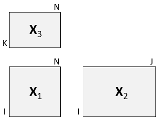
sim <- lplsData(I = 30, N = 20, J = 5, K = 6, ncomp = 2)
X1  <- sim$X1; X2 <- sim$X2; X3 <- sim$X3
lp  <- lpls(X1,X2,X3) # exo-L-PLS

Vector of component names

Description

Convenience function for creating a vector of component names based on the dimensions the input object (matrix or object having a score function).

Usage

compnames(object, comps, explvar = FALSE, ...)

Arguments

Details

This is a copy of compnames from the pls package to work with multiblock objects.

Value

A character vector of component names.

Distinctive and Common Components with SCA - DISCO

Description

This is a wrapper for the DISCOsca function by Zhengguo Gu for computing DISCO.

Usage

disco(X, ncomp = 2, ...)

Arguments

Details

DISCO is a restriction of SCA where Alternating Least Squares is used for estimation of loadings and scores. The SCA solution is rotated towards loadings (in sample linked mode) which are filled with zeros in a pattern resembling distinct, local and common components. When used in sample linked mode and only selecting distinct components, it shares a resemblance to SO-PLS, only in an unsupervised setting. Explained variances are computed as proportion of block variation explained by scores*loadings'.

Value

multiblock object including relevant scores and loadings. Relevant plotting functions: multiblock_plots and result functions: multiblock_results.

References

Schouteden, M., Van Deun, K., Wilderjans, T. F., & Van Mechelen, I. (2014). Performing DISCO-SCA to search for distinctive and common information in linked data. Behavior research methods, 46(2), 576-587.

See Also

Overviews of available methods, multiblock, and methods organised by main structure: basic, unsupervised, asca, supervised and complex.

Examples

data(potato)
potList <- as.list(potato[c(1,2,9)])
pot.disco  <- disco(potList)
plot(scores(pot.disco), labels="names")

Dummy-coding of a single vector

Description

Flexible dummy-coding allowing for all R's built-in types of contrasts and optional dropping of a factor level to reduce rank defficiency probability.

Usage

dummycode(Y, contrast = "contr.sum", drop = TRUE)

Arguments

Value

matrix made by dummy-coding the input vector.

Examples

vec <- c("a","a","b","b","c","c")
dummycode(vec)

Explained predictor variance

Description

Extraction and/or computation of explained variances for various object classes in the multiblock package.

Usage

explvar(object)

Arguments

Value

A vector of component-wise explained variances for predictors.

Examples

data(potato)
so <- sopls(Sensory ~ Chemical + Compression, data=potato, ncomp=c(10,10), 
            max_comps=10)
explvar(so)

Extracting the Extended Model Frame from a Formula or Fit

Description

This function attempts to apply model.frame and extend the result with columns of interactions.

Usage

extended.model.frame(formula, data, ..., sep = ".")

Arguments

Value

A data.frame that includes everything a model.frame does plus interaction terms.

Examples

dat <- data.frame(Y = c(1,2,3,4,5,6), 
                  X = factor(LETTERS[c(1,1,2,2,3,3)]), 
                  W = factor(letters[c(1,2,1,2,1,2)]))
extended.model.frame(Y ~ X*W, dat)

Generalized Canonical Analysis - GCA

Description

This is an interface to both SVD-based (default) and RGCCA-based GCA (wrapping the RGCCA::rgcca function)

Usage

gca(X, ncomp = "max", svd = TRUE, tol = 10^-12, corrs = TRUE, ...)

Arguments

Details

GCA is a generalisation of Canonical Correlation Analysis to handle three or more blocks. There are several ways to generalise, and two of these are available through gca. The default is an SVD based approach estimating a common subspace and measuring mean squared correlation to this. An alternative approach is available through RGCCA. For the SVD based approach, the ncomp parameter controls the block-wise decomposition while the following the consensus decomposition is limited to the minimum number of components from the individual blocks.

Value

multiblock object including relevant scores and loadings. Relevant plotting functions: multiblock_plots and result functions: multiblock_results. blockCoef contains canonical coefficients, while blockDecomp contains decompositions of each block.

References

• Carroll, J. D. (1968). Generalization of canonical correlation analysis to three or more sets of variables. Proceedings of the American Psychological Association, pages 227-22.

• Van der Burg, E. and Dijksterhuis, G. (1996). Generalised canonical analysis of individual sensory profiles and instrument data, Elsevier, pp. 221–258.

See Also

Overviews of available methods, multiblock, and methods organised by main structure: basic, unsupervised, asca, supervised and complex. Common functions for computation and extraction of results and plotting are found in multiblock_results and multiblock_plots, respectively.

Examples

data(potato)
potList <- as.list(potato[c(1,2,9)])
pot.gca <- gca(potList)
plot(scores(pot.gca), labels="names")

Generalized Procrustes Analysis - GPA

Description

This is a wrapper for the FactoMineR::GPA function for computing GPA.

Usage

gpa(X, graph = FALSE, ...)

Arguments

Details

GPA is a generalisation of Procrustes analysis, where one matrix is scaled and rotated to be as similar as possible to another one. Through the generalisation, individual scaling and rotation of each input matrix is performed against a common representation which is estimated in an iterative manner.

Value

multiblock object including relevant scores and loadings. Relevant plotting functions: multiblock_plots and result functions: multiblock_results.

References

Gower, J. C. (1975). Generalized procrustes analysis. Psychometrika. 40: 33–51.

See Also

Overviews of available methods, multiblock, and methods organised by main structure: basic, unsupervised, asca, supervised and complex. Common functions for computation and extraction of results and plotting are found in multiblock_results and multiblock_plots, respectively.

Examples

data(potato)
potList <- as.list(potato[c(1,2,9)])
pot.gpa    <- gpa(potList)
plot(scores(pot.gpa), labels="names")

Generalised Singular Value Decomposition - GSVD

Description

This is a wrapper for the geigen::gsvd function for computing GSVD.

Usage

gsvd(X)

Arguments

Details

GSVD is a generalisation of SVD to two variable-linked matrices where common loadings and block-wise scores are estimated.

Value

multiblock object with associated with printing, scores, loadings. Relevant plotting functions: multiblock_plots and result functions: multiblock_results.

References

Van Loan, C. (1976) Generalizing the singular value decomposition. SIAM Journal on Numerical Analysis, 13, 76–83.

See Also

Overviews of available methods, multiblock, and methods organised by main structure: basic, unsupervised, asca, supervised and complex. Common functions for computation and extraction of results and plotting are found in multiblock_results and multiblock_plots, respectively.

Examples

data(potato)
X <- potato$Chemical

gsvd.pot <- gsvd(lapply(potato[3:4], t))

Higher Order Generalized SVD - HOGSVD

Description

This is a simple implementation for computing HOGSVD

Usage

hogsvd(X)

Arguments

Details

HOGSVD is a generalisation of SVD to two or more blocks. It finds a common set of loadings across blocks and individual sets of scores per block.

Value

multiblock object including relevant scores and loadings. Relevant plotting functions: multiblock_plots and result functions: multiblock_results.

References

Ponnapalli, S. P., Saunders, M. A., Van Loan, C. F., & Alter, O. (2011). A higher-order generalized singular value decomposition for comparison of global mRNA expression from multiple organisms. PloS one, 6(12), e28072.

See Also

Overviews of available methods, multiblock, and methods organised by main structure: basic, unsupervised, asca, supervised and complex. Common functions for computation and extraction of results and plotting are found in multiblock_results and multiblock_plots, respectively.

Examples

data(candies)
candyList <- lapply(1:nlevels(candies$candy),function(x)candies$assessment[candies$candy==x,])
can.hogsvd <- hogsvd(candyList)
scoreplot(can.hogsvd, block=1, labels="names")

Hierarchical Principal component analysis - HPCA

Description

This is a wrapper for the RGCCA::rgcca function for computing HPCA.

Usage

hpca(X, ncomp = 2, scale = FALSE, verbose = FALSE, ...)

Arguments

Details

HPCA is a hierarchical PCA analysis which combines two or more blocks into a two-level decomposition with block-wise loadings and scores and superlevel common loadings and scores. The method is closely related to the supervised method MB-PLS in structure.

Value

multiblock object including relevant scores and loadings. Relevant plotting functions: multiblock_plots and result functions: multiblock_results.

References

Westerhuis, J.A., Kourti, T., and MacGregor,J.F. (1998). Analysis of multiblock and hierarchical PCA and PLS models. Journal of Chemometrics, 12, 301–321.

See Also

Overviews of available methods, multiblock, and methods organised by main structure: basic, unsupervised, asca, supervised and complex. Common functions for computation and extraction of results and plotting are found in multiblock_results and multiblock_plots, respectively.

Examples

data(potato)
potList <- as.list(potato[c(1,2,9)])
pot.hpca   <- hpca(potList)
plot(scores(pot.hpca), labels="names")

Inter-battery Factor Analysis - IFA

Description

This is a wrapper for the RGCCA::rgcca function for computing IFA.

Usage

ifa(X, ncomp = 1, scale = FALSE, verbose = FALSE, ...)

Arguments

Details

IFA rotates two matrices to align one or more factors against each other, maximising correlations.

Value

multiblock object with associated with printing, scores, loadings. Relevant plotting functions: multiblock_plots and result functions: multiblock_results.

References

Tucker, L. R. (1958). An inter-battery method of factor analysis. Psychometrika, 23(2), 111-136.

See Also

Overviews of available methods, multiblock, and methods organised by main structure: basic, unsupervised, asca, supervised and complex. Common functions for computation and extraction of results and plotting are found in multiblock_results and multiblock_plots, respectively.

Examples

data(potato)
X <- potato$Chemical

ifa.pot  <- ifa(potato[1:2])

Joint and Individual Variation Explained - JIVE

Description

This is a wrapper for the r.jive::jive function for computing JIVE.

Usage

jive(X, ...)

Arguments

Details

Jive performs a decomposition of the variation in two or more blocks into low-dimensional representations of individual and joint variation plus residual variation.

Value

multiblock object including relevant scores and loadings. Relevant plotting functions: multiblock_plots and result functions: multiblock_results.

References

Lock, E., Hoadley, K., Marron, J., and Nobel, A. (2013) Joint and individual variation explained (JIVE) for integrated analysis of multiple data types. Ann Appl Stat, 7 (1), 523–542.

See Also

Overviews of available methods, multiblock, and methods organised by main structure: basic, unsupervised, asca, supervised and complex.

Examples

 # Too time consuming for testing
  data(candies)
  candyList <- lapply(1:nlevels(candies$candy),function(x)candies$assessment[candies$candy==x,])
  can.jive  <- jive(candyList)
  summary(can.jive)

L-PLS regression

Description

Simultaneous decomposition of three blocks connected in an L pattern.

Usage

lpls(
  X1,
  X2,
  X3,
  ncomp = 2,
  doublecenter = TRUE,
  scale = c(FALSE, FALSE, FALSE),
  type = c("exo"),
  impute = FALSE,
  niter = 25,
  subsetX2 = NULL,
  subsetX3 = NULL,
  ...
)

Arguments

Details

Two versions of L-PLS are available: exo- and endo-L-PLS which assume an outward or inward relationship between the main block X1 and the two other blocks X2 and X3.

The exo_ort algorithm returns orthogonal scores and should be chosen for visual exploration in correlation loading plots. If exo-L-PLS with prediction is the main purpose of the model then the non-orthogonal exo type L-PLS should be chosen for which the predict function has prediction implemented.

Value

An object of type lpls and multiblock containing all results from the L-PLS analysis. The object type lpls is associated with functions for correlation loading plots, prediction and cross-validation. The type multiblock is associated with the default functions for result presentation (multiblock_results) and plotting (multiblock_plots).

Author(s)

Solve Sæbø (adapted by Kristian Hovde Liland)

References

• Martens, H., Anderssen, E., Flatberg, A.,Gidskehaug, L.H., Høy, M., Westad, F.,Thybo, A., and Martens, M. (2005). Regression of a data matrix on descriptors of both its rows and of its columns via latent variables: L-PLSR. Computational Statistics & Data Analysis, 48(1), 103 – 123.

• Sæbø, S., Almøy, T., Flatberg, A., Aastveit, A.H., and Martens, H. (2008). LPLS-regression: a method for prediction and classification under the influence of background information on predictor variables. Chemometrics and Intelligent Laboratory Systems, 91, 121–132.

• Sæbø, S., Martens, M. and Martens H. (2010) Three-block data modeling by endo- and exo-LPLS regression. In Handbook of Partial Least Squares: Concepts, Methods and Applications. Esposito Vinzi, V.; Chin, W.W.; Henseler, J.; Wang, H. (Eds.). Springer.

See Also

Overviews of available methods, multiblock, and methods organised by main structure: basic, unsupervised, asca, supervised and complex. Functions for computation and extraction of results and plotting are found in lpls_results.

Examples

# Simulate data set
sim <- lplsData(I = 30, N = 20, J = 5, K = 6, ncomp = 2)
X1  <- sim$X1; X2 <- sim$X2; X3 <- sim$X3
lp  <- lpls(X1,X2,X3) # exo-L-PLS

L-PLS data simulation for exo-type analysis

Description

Three data blocks are simulated to express covariance in an exo-L-PLS direction (see lpls. Dimensionality and number of underlying components can be controlled.

Usage

lplsData(I = 30, N = 20, J = 5, K = 6, ncomp = 2)

Arguments

Value

A list of three matrices with dimensions matching in an L-shape.

Author(s)

Solve Sæbø (adapted by Kristian Hovde Liland)

See Also

Overviews of available methods, multiblock, and methods organised by main structure: basic, unsupervised, asca, supervised and complex.

Examples

lp <- lplsData(I = 30, N = 20, J = 5, K = 6, ncomp = 2)
names(lp)

Result functions for L-PLS objects (lpls)

Description

Correlation loading plot, prediction and cross-validation for L-PLS models with class lpls.

Usage

## S3 method for class 'lpls'
plot(
  x,
  comps = c(1, 2),
  doplot = c(TRUE, TRUE, TRUE),
  level = c(2, 2, 2),
  arrow = c(1, 0, 1),
  xlim = c(-1, 1),
  ylim = c(-1, 1),
  samplecol = 4,
  pathcol = 2,
  varcol = "grey70",
  varsize = 1,
  sampleindex = 1:dim(x$corloadings$R22)[1],
  pathindex = 1:dim(x$corloadings$R3)[1],
  varindex = 1:dim(x$corloadings$R21)[1],
  ...
)

## S3 method for class 'lpls'
predict(
  object,
  X1new = NULL,
  X2new = NULL,
  X3new = NULL,
  exo.direction = c("X2", "X3"),
  ...
)

lplsCV(object, segments1 = NULL, segments2 = NULL, trace = TRUE)

Arguments

Value

Nothing is return for plotting (plot.lpls), predicted values are returned for predictions (predict.lpls) and cross-validation metrics are returned for for cross-validation (lplsCV).

See Also

Overviews of available methods, multiblock, and methods organised by main structure: basic, unsupervised, asca, supervised and complex.

Examples

# Simulate data set
sim <- lplsData(I = 30, N = 20, J = 5, K = 6, ncomp = 2)
X1  <- sim$X1; X2 <- sim$X2; X3 <- sim$X3

# exo-L-PLS:
lp.exo  <- lpls(X1,X2,X3, ncomp = 2)
# Predict X1
pred.exo.X2 <- predict(lp.exo, X1new = X1, exo.direction = "X2")
# Predict X3
pred.exo.X2 <- predict(lp.exo, X1new = X1, exo.direction = "X3")

# endo-L-PLS:
lp.endo <- lpls(X1,X2,X3, ncomp = 2, type = "endo")
# Predict X1 from X2 and X3 (in this case fitted values):
pred.endo.X1 <- predict(lp.endo, X2new = X2, X3new = X3)

# LOO cross-validation horizontally
lp.cv1 <- lplsCV(lp.exo, segments1 = as.list(1:dim(X1)[1]))

# LOO cross-validation vertically
lp.cv2 <- lplsCV(lp.exo, segments2 = as.list(1:dim(X1)[2]))

# Three-fold CV, horizontal
lp.cv3 <- lplsCV(lp.exo, segments1 = as.list(1:10, 11:20, 21:30))

Måge plot

Description

Måge plot for SO-PLS (sopls) cross-validation visualisation.

Usage

maage(
  object,
  expl_var = TRUE,
  pure.trace = FALSE,
  pch = 20,
  xlab = "# components",
  ylab = ifelse(expl_var, "Explained variance (%)", "RMSECV"),
  xlim = NULL,
  ylim = NULL,
  cex.text = 0.8,
  ...
)

maageSeq(
  object,
  compSeq = TRUE,
  expl_var = TRUE,
  pch = 20,
  xlab = "# components",
  ylab = ifelse(expl_var, "Explained variance (%)", "RMSECV"),
  xlim = NULL,
  ylim = NULL,
  cex.text = 0.8,
  col = "gray",
  col.block = c("red", "blue", "darkgreen", "purple", "black", "red", "blue",
    "darkgreen"),
  ...
)

Arguments

Details

This function can either be used for global optimisation across blocks or sequential optimisation, using maageSeq. The examples below show typical usage.

Value

The maage plot has no return.

See Also

Overviews of available methods, multiblock, and methods organised by main structure: basic, unsupervised, asca, supervised and complex.

Examples

data(wine)
ncomp <- unlist(lapply(wine, ncol))[-5]
so.wine <- sopls(`Global quality` ~ ., data=wine, ncomp=ncomp, 
            max_comps=10, validation="CV", segments=10)
maage(so.wine)

# Sequential search for optimal number of components per block
old.par <- par(mfrow=c(2,2), mar=c(3,3,0.5,1), mgp=c(2,0.7,0))
maageSeq(so.wine)
maageSeq(so.wine, 2)
maageSeq(so.wine, c(2,1))
maageSeq(so.wine, c(2,1,1))
par(old.par)

Multiblock Partial Least Squares - MB-PLS

Description

A function computing MB-PLS scores, loadings, etc. on the super-level and block-level.

Usage

mbpls(
  formula,
  data,
  subset,
  na.action,
  X = NULL,
  Y = NULL,
  ncomp = 1,
  scale = FALSE,
  blockScale = c("sqrtnvar", "ssq", "none"),
  ...
)

Arguments

Details

MB-PLS is the prototypical component based supervised multiblock method. It was originally formulated as a two-level method with a block-level and a super-level, but it was later discovered that it could be expressed as an ordinary PLS on concatenated weighted X blocks followed by a simple loop for calculating block-level loading weights, loadings and scores. This implementation uses the plsr function on the scaled input blocks (1/sqrt(ncol)) enabling all summaries and plots from the pls package.

Block weighting is performed after scaling all variables and is by default "sqrtnvar": 1/sqrt(ncol(X[[i]])) in each block. Alternatives are "ssq": 1/norm(X[[i]], "F")^2 and "none": 1/1. Finally, if a numeric vector is supplied, it will be used to scale the blocks after "ssq" scaling, i.e., Z[[i]] = X[[i]] / norm(X[[i]], "F")^2 * blockScale[i].

Value

multiblock, mvr object with super-scores, super-loadings, block-scores and block-loading, and the underlying mvr (PLS) object for the super model, with all its result and plot possibilities. Relevant plotting functions: multiblock_plots and result functions: multiblock_results.

References

• Wangen, L.E. and Kowalski, B.R. (1988). A multiblock partial least squares algorithm for investigating complex chemical systems. Journal of Chemometrics, 3, 3–20.

• Westerhuis, J.A., Kourti, T., and MacGregor,J.F. (1998). Analysis of multiblock and hierarchical PCA and PLS models. Journal of Chemometrics, 12, 301–321.

See Also

Overviews of available methods, multiblock, and methods organised by main structure: basic, unsupervised, asca, supervised and complex.

Examples

data(potato)
# Formula interface
mb <- mbpls(Sensory ~ Chemical+Compression, data=potato, ncomp = 5)

# ... or X and Y
mb.XY <- mbpls(X=potato[c('Chemical','Compression')], Y=potato[['Sensory']], ncomp = 5)
identical(mb$scores, mb.XY$scores)
print(mb)
scoreplot(mb, labels="names") # Exploiting mvr object structure from pls package

# Block scaling with emphasis on first block
mbs <- mbpls(Sensory ~ Chemical+Compression, data=potato, ncomp = 5, blockScale = c(10, 1))
scoreplot(mbs, labels="names") # Exploiting mvr object structure from pls package

Multiblock Redundancy Analysis - mbRDA

Description

This is a wrapper for the ade4::mbpcaiv function for computing mbRDA.

Usage

mbrda(formula, data, subset, na.action, X = NULL, Y = NULL, ncomp = 1, ...)

Arguments

Details

mbRDA is a multiblock formulation of Redundancy (Data) Analysis. RDA is theoretically between PLS and GCA. Like GCA, RDA does not consider correlations within X, but like PLS it does consider correlations within Y. RDA can also be viewed as a PCR of Y constrained to have scores that are also linear combinations of X. If the adegraphics package is attached, a nice overview can be plotted as plot(mbr$mbpcaiv) following the example below.

Value

multiblock, mvr object with scores, block-scores and block-loading. Relevant plotting functions: multiblock_plots and result functions: multiblock_results.

References

Bougeard, S., Qannari, E.M., Lupo, C., andHanafi, M. (2011). From Multiblock Partial Least Squares to Multiblock Redundancy Analysis. A Continuum Approach. Informatica, 22(1), 11–26.

See Also

Overviews of available methods, multiblock, and methods organised by main structure: basic, unsupervised, asca, supervised and complex.

Examples

# Convert data.frame with AsIs objects to list of matrices
data(potato)
potatoList <- lapply(potato, unclass)

mbr <- mbrda(Sensory ~ Chemical + Compression, data = potatoList, ncomp = 10)
mbr.XY <- mbrda(X = potatoList[c('Chemical','Compression')], Y = potatoList[['Sensory']], 
                ncomp = 10)
print(mbr)
scoreplot(mbr) # Exploiting mvr object structure from pls package

Multiple Co-Inertia Analysis - MCOA

Description

This is a wrapper for the RGCCA::rgcca function for computing MCOA.

Usage

mcoa(X, ncomp = 2, scale = FALSE, verbose = FALSE, ...)

Arguments

Details

MCOA resembles GCA and MFA in that it creates a set of reference scores, for which each block's individual scores should correlate maximally too, but also the variance within each block should be taken into account. A single component solution is equivalent to a PCA on concatenated blocks scaled by the so called inverse inertia.

Value

multiblock object including relevant scores and loadings. Relevant plotting functions: multiblock_plots and result functions: multiblock_results.

References

• Le Roux; B. and H. Rouanet (2004). Geometric Data Analysis, From Correspondence Analysis to Structured Data Analysis. Dordrecht. Kluwer: p.180.

• Greenacre, Michael and Blasius, Jörg (editors) (2006). Multiple Correspondence Analysis and Related Methods. London: Chapman & Hall/CRC.

See Also

Overviews of available methods, multiblock, and methods organised by main structure: basic, unsupervised, asca, supervised and complex. Common functions for computation and extraction of results and plotting are found in multiblock_results and multiblock_plots, respectively.

Examples

data(potato)
potList <- as.list(potato[c(1,2,9)])
pot.mcoa   <- mcoa(potList)
plot(scores(pot.mcoa), labels="names")

Colour palette generation from matrix of RGB values

Description

Colour palette generation from matrix of RGB values

Usage

mcolors(
  n,
  colmatrix = matrix(c(0, 0, 1, 1, 1, 1, 1, 0, 0), 3, 3, byrow = TRUE)
)

Arguments

Value

A vector of n colours in hexadecimal RGB format.

Examples

mcolors(5)

Multiple Factor Analysis - MFA

Description

This is a wrapper for the FactoMineR::MFA function for computing MFA.

Usage

mfa(X, type = rep("c", length(X)), graph = FALSE, ...)

Arguments

Details

MFA is a methods typically used to compare several equally sized matrices. It is often used in sensory analyses, where matrices consist of sensory characteristics and products, and each assessor generates one matrix each. In its basic form, MFA scales all matrices by their largest eigenvalue, concatenates them and performs PCA on the result. There are several possibilities for plots and inspections of the model, handling of categorical and continuous inputs etc. connected to MFA.

Value

multiblock object including relevant scores and loadings. Relevant plotting functions: multiblock_plots and result functions: multiblock_results.

References

Pagès, J. (2005). Collection and analysis of perceived product inter-distances using multiple factor analysis: Application to the study of 10 white wines from the Loire valley. Food Quality and Preference, 16(7), 642–649.

See Also

Overviews of available methods, multiblock, and methods organised by main structure: basic, unsupervised, asca, supervised and complex. Common functions for computation and extraction of results and plotting are found in multiblock_results and multiblock_plots, respectively.

Examples

data(potato)
potList <- as.list(potato[c(1,2,9)])
pot.mfa    <- mfa(potList)
if(interactive()){
  plot(pot.mfa$MFA)
}

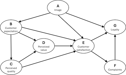
ECSI Mobile Mobile Phone Provider Dataset

Description

Mobile data questionnaire often used as an example in path modelling. All the items are scaled from 1 to 10. Score 1 expresses a very negative point of view on the product while score 10 a very positive opinion. For details, see the original publication.

Usage

data(mobile)

Format

A data.frame having 250 rows and 7 variables:

A

Image

B

Customer expectation

C

Perceived quality

D

Perceived value

E

Customer satisfaction

F

Customer complaints

G

Customer loyalty

References

Tenenhaus M, Esposito Vinzi V, Chatelin YM, Lauro C. PLS path modeling. Comput Stat Data Anal. 2005;48(1):159‐205.

Plot Functions for Multiblock Objects

Description

Plotting procedures for multiblock objects.

Usage

## S3 method for class 'multiblock'
scoreplot(
  object,
  comps = 1:2,
  block = 0,
  labels,
  identify = FALSE,
  type = "p",
  xlab,
  ylab,
  main,
  ...
)

## S3 method for class 'multiblock'
loadingplot(
  object,
  comps = 1:2,
  block = 0,
  scatter = TRUE,
  labels,
  identify = FALSE,
  type,
  lty,
  lwd = NULL,
  pch,
  cex = NULL,
  col,
  legendpos,
  xlab,
  ylab,
  main,
  pretty.xlabels = TRUE,
  xlim,
  ...
)

loadingweightplot(object, main = "Loading weights", ...)

## S3 method for class 'multiblock'
biplot(
  x,
  block = 0,
  comps = 1:2,
  which = c("x", "y", "scores", "loadings"),
  var.axes = FALSE,
  xlabs,
  ylabs,
  main,
  ...
)

corrplot(object, ...)

## Default S3 method:
corrplot(object, ...)

## S3 method for class 'mvr'
corrplot(object, ...)

## S3 method for class 'multiblock'
corrplot(
  object,
  comps = 1:2,
  labels = TRUE,
  col = 1:5,
  plotx = TRUE,
  ploty = TRUE,
  blockScores = FALSE,
  ...
)

Arguments

Details

Plot functions for scores, loadings and loading.weights based on the functions found in the pls package.

Value

These plotting routines only generate plots and return no values.

See Also

Overviews of available methods, multiblock, and methods organised by main structure: basic, unsupervised, asca, supervised and complex. Common functions for computation and extraction of results are found in multiblock_results.

Examples

data(wine)
sc <- sca(wine[c('Smell at rest', 'View', 'Smell after shaking')], ncomp = 4)
loadingplot(sc, block = 1, labels = "names", scatter = TRUE)
scoreplot(sc, labels = "names")
corrplot(sc)

data(potato)
so <- sopls(Sensory ~ NIRraw + Chemical + Compression, data=potato, ncomp = c(2,2,2), 
            max_comps = 6, validation = "CV", segments = 10)
scoreplot(so, ncomp = c(2,1), block = 3, labels = "names")
corrplot(pcp(so, ncomp = c(2,2,2)))

Result Functions for Multiblock Objects

Description

Standard result computation and extraction functions for multiblock objects.

Usage

## S3 method for class 'multiblock'
scores(object, block = 0, ...)

## S3 method for class 'multiblock'
loadings(object, block = 0, ...)

## S3 method for class 'multiblock'
print(x, ...)

## S3 method for class 'multiblock'
summary(object, ...)

Arguments

Details

Usage of the functions are shown using generics in the examples below. Object printing and summary are available through: print.multiblock and summary.multiblock. Scores and loadings have their own extensions of scores() and loadings() throught scores.multiblock and loadings.multiblock.

Value

Scores or loadings are returned by scores.multiblock and loadings.multiblock, while print and summary methods invisibly returns the object.

See Also

Overviews of available methods, multiblock, and methods organised by main structure: basic, unsupervised, asca, supervised and complex. Common functions for plotting are found in multiblock_plots, respectively.

Examples

data(wine)
sc <- sca(wine[c('Smell at rest', 'View', 'Smell after shaking')], ncomp = 4)
print(sc)
summary(sc)
head(loadings(sc, block = 1))
head(scores(sc))

MSEP, RMSEP and R2 of the MB-PLS model

Description

Functions to estimate the mean squared error of prediction (MSEP), root mean squared error of prediction (RMSEP) and R^2 (A.K.A. coefficient of multiple determination) for a fitted MB-PLS models. Test-set, cross-validation and calibration-set estimates are implemented.

Usage

## S3 method for class 'mbpls'
R2(
  object,
  estimate,
  newdata,
  ncomp = 1:object$ncomp,
  comps,
  intercept = TRUE,
  se = FALSE,
  ...
)

## S3 method for class 'mbpls'
MSEP(
  object,
  estimate,
  newdata,
  ncomp = 1:object$ncomp,
  comps,
  intercept = TRUE,
  se = FALSE,
  ...
)

## S3 method for class 'mbpls'
RMSEP(object, ...)

Arguments

Details

RMSEP simply calls MSEP and takes the square root of the estimates. It therefore accepts the same arguments as MSEP.

Several estimators can be used. "train" is the training or calibration data estimate, also called (R)MSEC. For R2, this is the unadjusted R^2. It is overoptimistic and should not be used for assessing models. "CV" is the cross-validation estimate, and "adjCV" (for RMSEP and MSEP) is the bias-corrected cross-validation estimate. They can only be calculated if the model has been cross-validated. Finally, "test" is the test set estimate, using newdata as test set.

Which estimators to use is decided as follows (see below for pls:mvrValstats). If estimate is not specified, the test set estimate is returned if newdata is specified, otherwise the CV and adjusted CV (for RMSEP and MSEP) estimates if the model has been cross-validated, otherwise the training data estimate. If estimate is "all", all possible estimates are calculated. Otherwise, the specified estimates are calculated.

Several model sizes can also be specified. If comps is missing (or is NULL), length(ncomp) models are used, with ncomp[1] components, ..., ncomp[length(ncomp)] components. Otherwise, a single model with the components comps[1], ..., comps[length(comps)] is used. If intercept is TRUE, a model with zero components is also used (in addition to the above).

The R^2 values returned by "R2" are calculated as 1 - SSE/SST, where SST is the (corrected) total sum of squares of the response, and SSE is the sum of squared errors for either the fitted values (i.e., the residual sum of squares), test set predictions or cross-validated predictions (i.e., the PRESS). For estimate = "train", this is equivalent to the squared correlation between the fitted values and the response. For estimate = "train", the estimate is often called the prediction R^2.

mvrValstats is a utility function that calculates the statistics needed by MSEP and R2. It is not intended to be used interactively. It accepts the same arguments as MSEP and R2. However, the estimate argument must be specified explicitly: no partial matching and no automatic choice is made. The function simply calculates the types of estimates it knows, and leaves the other untouched.

Value

mvrValstats returns a list with components

SSE

three-dimensional array of SSE values. The first dimension is the different estimators, the second is the response variables and the third is the models.

SST

matrix of SST values. The first dimension is the different estimators and the second is the response variables.

nobj

a numeric vector giving the number of objects used for each estimator.

comps

the components specified, with 0 prepended if intercept is TRUE.

cumulative

TRUE if comps was NULL or not specified.

The other functions return an object of class "mvrVal", with components

val

three-dimensional array of estimates. The first dimension is the different estimators, the second is the response variables and the third is the models.

type

"MSEP", "RMSEP" or "R2".

comps

the components specified, with 0 prepended if intercept is TRUE.

cumulative

TRUE if comps was NULL or not specified.

call

the function call

Author(s)

Kristian Hovde Liland

References

Mevik, B.-H., Cederkvist, H. R. (2004) Mean Squared Error of Prediction (MSEP) Estimates for Principal Component Regression (PCR) and Partial Least Squares Regression (PLSR). Journal of Chemometrics, 18(9), 422–429.

See Also

mbpls

Examples

data(oliveoil, package = "pls")
mod <- pls::plsr(sensory ~ chemical, ncomp = 4, data = oliveoil, validation = "LOO")
RMSEP(mod)
## Not run: plot(R2(mod))

Principal Component Analysis - PCA

Description

This is a wrapper for the pls::PCR function for computing PCA.

Usage

pca(X, scale = FALSE, ncomp = 1, ...)

Arguments

Details

PCA is a method for decomposing a matrix into subspace components with sample scores and variable loadings. It can be formulated in various ways, but the standard formulation uses singular value decomposition to create scores and loadings. PCA is guaranteed to be the optimal way of extracting orthogonal subspaces from a matrix with regard to the amount of explained variance per component.

Value

multiblock object with scores, loadings, mean X values and explained variances. Relevant plotting functions: multiblock_plots and result functions: multiblock_results.

References

Pearson, K. (1901) On lines and planes of closest fit to points in space. Philosophical Magazine, 2, 559–572.

See Also

Overviews of available methods, multiblock, and methods organised by main structure: basic, unsupervised, asca, supervised and complex. Common functions for computation and extraction of results and plotting are found in multiblock_results and multiblock_plots, respectively.

Examples

data(potato)
X <- potato$Chemical

pca.pot  <- pca(X, ncomp = 2)

PCA-GCA

Description

PCA-GCA is a methods which aims at estimating subspaces of common, local and distinct variation from two or more blocks.

Usage

pcagca(
  X,
  commons = 2,
  auto = TRUE,
  auto.par = list(explVarLim = 40, rLim = 0.8),
  manual.par = list(ncomp = 0, ncommon = 0),
  tol = 10^-12
)

Arguments

Details

The name PCA-GCA comes from the process of first applying PCA to each block, then using GCA to estimate local and common components, and finally orthogonalising the block-wise scores on the local/common ones and re-estimating these to obtain distinct components. The procedure is highly similar to the supervised method PO-PLS, where the PCA steps are exchanged with PLS.

Value

multiblock object including relevant scores and loadings. Relevant plotting functions: multiblock_plots and result functions: multiblock_results. Distinct components are marked as 'D(x), Comp c' for block x and component c while local and common components are marked as "C(x1, x2), Comp c", where x1 and x2 (and more) are block numbers.

References

Smilde, A., Måge, I., Naes, T., Hankemeier, T.,Lips, M., Kiers, H., Acar, E., and Bro, R.(2017). Common and distinct components in data fusion. Journal of Chemometrics, 31(7), e2900.

See Also

Overviews of available methods, multiblock, and methods organised by main structure: basic, unsupervised, asca, supervised and complex. Common functions for computation and extraction of results and plotting are found in multiblock_results and multiblock_plots, respectively.

Examples

data(potato)
potList <- as.list(potato[c(1,2,9)])
pot.pcagca <- pcagca(potList)

# Show origin and type of all components
lapply(pot.pcagca$blockScores,colnames)

# Basic multiblock plot
plot(scores(pot.pcagca, block=2), comps=1, labels="names")

Parallel and Orthogonalised Partial Least Squares - PO-PLS

Description

This is a basic implementation of PO-PLS with manual and automatic component selections.

Usage

popls(
  X,
  Y,
  commons = 2,
  auto = TRUE,
  auto.par = list(explVarLim = 40, rLim = 0.8),
  manual.par = list(ncomp = rep(0, length(X)), ncommon = list())
)

Arguments

Details

PO-PLS decomposes a set of input data blocks into common, local and distinct components through a process involving pls and gca. The rLim parameter is a lower bound for the GCA correlation when building common components, while explVarLim is the minimum explained variance for common components and unique components.

Value

A multiblock object with block-wise, local and common loadings and scores. Relevant plotting functions: multiblock_plots and result functions: multiblock_results.

References

• I Måge, BH Mevik, T Næs. (2008). Regression models with process variables and parallel blocks of raw material measurements. Journal of Chemometrics: A Journal of the Chemometrics Society 22 (8), 443-456

• I Måge, E Menichelli, T Næs (2012). Preference mapping by PO-PLS: Separating common and unique information in several data blocks. Food quality and preference 24 (1), 8-16

See Also

Overviews of available methods, multiblock, and methods organised by main structure: basic, unsupervised, asca, supervised and complex. Common functions for computation and extraction of results and plotting are found in multiblock_results and multiblock_plots, respectively.

Examples

data(potato)

# Automatic analysis
pot.po.auto <- popls(potato[1:3], potato[['Sensory']][,1])
pot.po.auto$explVar

# Manual choice of up to 5 components for each block and 1, 0, and 2 blocks,
# respectively from the (1,2), (1,3) and (2,3) combinations of blocks.
pot.po.man <- popls(potato[1:3], potato[['Sensory']][,1], auto=FALSE, 
                manual.par = list(ncomp=c(5,5,5), ncommon=c(1,0,2)))
pot.po.man$explVar

# Score plot for local (2,3) components
plot(scores(pot.po.man,3), comps=1:2, labels="names")

Sensory, rheological, chemical and spectroscopic analysis of potatoes.

Description

A dataset containing 9 blocks of measurements on 26 potatoes. Original dataset can be found at http://models.life.ku.dk/Texture_Potatoes. This version has been pre-processed as follows (corresponding to Liland et al. 2016):

• Variables containing NaN have been removed.

• Chemical and Compression blocks have been scaled by standard deviations.

• NIR blocks have been subjected to SNV (Standard Normal Variate).

Usage

data(potato)

Format

A data.frame having 26 rows and 9 variables:

Chemical

Matrix of chemical measurements

Compression

Matrix of rheological compression data

NIRraw

Matrix of near-infrared measurements of raw potatoes

NIRcooked

Matrix of near-infrared measurements of cooked potatoes

CPMGraw

Matrix of NMR (CPMG) measurements of raw potatoes

CPMGcooked

Matrix of NMR (CPMG) measurements of cooked potatoes

FIDraw

Matrix of NMR (FID) measurements of raw potatoes

FIDcooked

Matrix of NMR (FID) measurements of cooked potatoes

Sensory

Matrix of sensory assessments

References

• L.G.Thygesen, A.K.Thybo, S.B.Engelsen, Prediction of Sensory Texture Quality of Boiled Potatoes From Low-field1H NMR of Raw Potatoes. The Role of Chemical Constituents. LWT - Food Science and Technology 34(7), 2001, pp 469-477.

• Kristian Hovde Liland, Tormod Næs, Ulf Geir Indahl, ROSA – a fast extension of Partial Least Squares Regression for Multiblock Data Analysis, Journal of Chemometrics 30:11 (2016), pp. 651-662.

Predict Method for MBPLS

Description

Prediction for the mbpls (MBPLS) model. New responses or scores are predicted using a fitted model and a data.frame or list containing matrices of observations.

Usage

## S3 method for class 'mbpls'
predict(
  object,
  newdata,
  ncomp = 1:object$ncomp,
  comps,
  type = c("response", "scores"),
  na.action = na.pass,
  ...
)

Arguments

Details

When type is "response" (default), predicted response values are returned. If comps is missing (or is NULL), predictions for length(ncomp) models with ncomp[1] components, ncomp[2] components, etc., are returned. Otherwise, predictions for a single model with the exact components in comps are returned. (Note that in both cases, the intercept is always included in the predictions. It can be removed by subtracting the Ymeans component of the fitted model.)

When type is "scores", predicted score values are returned for the components given in comps. If comps is missing or NULL, ncomps is used instead.

Value

When type is "response", a three dimensional array of predicted response values is returned. The dimensions correspond to the observations, the response variables and the model sizes, respectively.

When type is "scores", a score matrix is returned.

Note

A warning message like ‘⁠'newdata' had 10 rows but variable(s) found have 106 rows⁠’ means that not all variables were found in the newdata data frame. This (usually) happens if the formula contains terms like yarn$NIR. Do not use such terms; use the data argument instead. See mvr for details.

Author(s)

Kristian Hovde Liland

See Also

mbpls

Examples

data(potato)
mb <- mbpls(Sensory ~ Chemical+Compression, data=potato, ncomp = 5, subset = 1:26 <= 18)
testdata <- subset(potato, 1:26 > 18)

# Predict response
yhat <- predict(mb, newdata = testdata)

# Predict scores and plot
scores <- predict(mb, newdata = testdata, type = "scores")
scoreplot(mb)
points(scores[,1], scores[,2], col="red")
legend("topright", legend = c("training", "test"), col=1:2, pch = 1)

Preprocessing of block data

Description

This is an interface to simplify preprocessing of one, a subset or all blocks in a multiblock object, e.g., a data.frame (see block.data.frame) or list. Several standard preprocessing methods are supplied in addition to letting the user supply it's own function.

Usage

block.preprocess(
  X,
  block = 1:length(X),
  fun = c("autoscale", "center", "scale", "SNV", "EMSC", "Fro", "FroSq", "SingVal"),
  ...
)

Arguments

Details

The fun parameter controls the type of preprocessing to be performed:

• autoscale: centre and scale each feature/variable.

• center: centre each feature/variable.

• scale: scale each feature/variable.

• SNV: Standard Normal Variate correction, i.e., centre and scale each sample across features/variables.

• EMSC: Extended Multiplicative Signal Correction defaulting to basic EMSC (2nd order polynomials). Further parameters are sent to EMSC::EMSC.

• Fro: Frobenius norm scaling of whole block.

• FroSq: Squared Frobenius norm scaling of whole block (sum of squared values).

• SingVal: Singular value scaling of whole block (first singular value).

• User defined: If a function is supplied, this will be applied to chosen blocks. Preprocessing can be done for all blocks or a subset. It can also be done in a series of operations to combine preprocessing techniques.

Value

The input multiblock object is preprocessed and returned.

See Also

Overviews of available methods, multiblock, and methods organised by main structure: basic, unsupervised, asca, supervised and complex. Common functions for computation and extraction of results and plotting are found in multiblock_results and multiblock_plots, respectively.

Examples

data(potato)
# Autoscale Chemical block
potato <- block.preprocess(potato, block = "Chemical", "autoscale")
# Apply SNV to NIR blocks
potato <- block.preprocess(potato, block = 3:4, "SNV")
# Centre Sensory block
potato <- block.preprocess(potato, block = "Sensory", "center")
# Scale all blocks to unit Frobenius norm
potato <- block.preprocess(potato, fun = "Fro")

# Effect of SNV
NIR <- (potato$NIRraw + rnorm(26)) * rnorm(26,1,0.2)
NIRc <- block.preprocess(list(NIR), fun = "SNV")[[1]]
old.par <- par(mfrow = c(2,1), mar = c(4,4,1,1))
matplot(t(NIR), type="l", main = "uncorrected", ylab = "")
matplot(t(NIRc), type="l", main = "corrected", ylab = "")
par(old.par)

Objects exported from other packages

Description

These objects are imported from other packages. Follow the links below to see their documentation.

HDANOVA

asca, loadingplot, permutationplot, scoreplot, timeplot

pls

MSEP, R2, RMSEP, coefplot, cvsegments, loading.weights, loadingplot, loadings, mvrValstats, pcr, plsr, predplot, scoreplot, scores, validationplot

Response Oriented Sequential Alternation - ROSA

Description

Formula based interface to the ROSA algorithm following the style of the pls package.

Usage

rosa(
  formula,
  ncomp,
  Y.add,
  common.comp = 1,
  data,
  subset,
  na.action,
  scale = FALSE,
  weights = NULL,
  validation = c("none", "CV", "LOO"),
  internal.validation = FALSE,
  fixed.block = NULL,
  design.block = NULL,
  canonical = TRUE,
  ...
)

Arguments

Details

ROSA is an opportunistic method sequentially selecting components from whichever block explains the response most effectively. It can be formulated as a PLS model on concatenated input block with block selection per component. This implementation adds several options that are not described in the literature. Most importantly, it opens for internal validation in the block selection process, making this more robust. In addition it handles design blocks explicitly, enables classification and secondary responses (CPLS), and definition of common components.

Value

An object of classes rosa and mvr having several associated printing (rosa_results) and plotting methods (rosa_plots).

References

Liland, K.H., Næs, T., and Indahl, U.G. (2016). ROSA - a fast extension of partial least squares regression for multiblock data analysis. Journal of Chemometrics, 30, 651–662, doi:10.1002/cem.2824.

See Also

Overviews of available methods, multiblock, and methods organised by main structure: basic, unsupervised, asca, supervised and complex. Common functions for computation and extraction of results and plotting are found in rosa_results and rosa_plots, respectively.

Examples

data(potato)
mod <- rosa(Sensory[,1] ~ ., data = potato, ncomp = 10, validation = "CV", segments = 5)
summary(mod)

# For examples of ROSA results and plotting see 
# ?rosa_results and ?rosa_plots.

Plotting functions for ROSA models

Description

Various plotting procedures for rosa objects.

Usage

## S3 method for class 'rosa'
image(
  x,
  type = c("correlation", "residual", "order"),
  ncomp = x$ncomp,
  col = mcolors(128),
  legend = TRUE,
  mar = c(5, 6, 4, 7),
  las = 1,
  ...
)

## S3 method for class 'rosa'
barplot(
  height,
  type = c("train", "CV"),
  ncomp = height$ncomp,
  col = mcolors(ncomp),
  ...
)

Arguments

Details

Usage of the functions are shown using generics in the examples below. image.rosa makes an image plot of each candidate score's correlation to the winner or the block-wise response residual. These plots can be used to find alternative block selection for tweaking the ROSA model. barplot.rosa makes barplot of block and component explained variances. loadingweightsplot is an adaptation of pls::loadingplot to plot loading weights.

Value

No return.

References

Liland, K.H., Næs, T., and Indahl, U.G. (2016). ROSA - a fast extension of partial least squares regression for multiblock data analysis. Journal of Chemometrics, 30, 651–662, doi:10.1002/cem.2824.

See Also

Overviews of available methods, multiblock, and methods organised by main structure: basic, unsupervised, asca, supervised and complex. Common functions for computation and extraction of results in rosa_results.

Examples

data(potato)
mod <- rosa(Sensory[,1] ~ ., data = potato, ncomp = 5)
image(mod)
barplot(mod)
loadingweightplot(mod)

Result functions for ROSA models

Description

Standard result computation and extraction functions for ROSA (rosa).

Usage

## S3 method for class 'rosa'
predict(
  object,
  newdata,
  ncomp = 1:object$ncomp,
  comps,
  type = c("response", "scores"),
  na.action = na.pass,
  ...
)

## S3 method for class 'rosa'
coef(object, ncomp = object$ncomp, comps, intercept = FALSE, ...)

## S3 method for class 'rosa'
print(x, ...)

## S3 method for class 'rosa'
summary(
  object,
  what = c("all", "validation", "training"),
  digits = 4,
  print.gap = 2,
  ...
)

blockexpl(object, ncomp = object$ncomp, type = c("train", "CV"))

## S3 method for class 'rosaexpl'
print(x, digits = 3, compwise = FALSE, ...)

rosa.classify(object, classes, newdata, ncomp, LQ)

## S3 method for class 'rosa'
scores(object, ...)

## S3 method for class 'rosa'
loadings(object, ...)

Arguments

Details

Usage of the functions are shown using generics in the examples below. Prediction, regression coefficients, object printing and summary are available through: predict.rosa, coef.rosa, print.rosa and summary.rosa. Explained variances are available (block-wise and global) through blockexpl and print.rosaexpl. Scores and loadings have their own extensions of scores() and loadings() throught scores.rosa and loadings.rosa. Finally, there is work in progress on classifcation support through rosa.classify.

When type is "response" (default), predicted response values are returned. If comps is missing (or is NULL), predictions for length(ncomp) models with ncomp[1] components, ncomp[2] components, etc., are returned. Otherwise, predictions for a single model with the exact components in comps are returned. (Note that in both cases, the intercept is always included in the predictions. It can be removed by subtracting the Ymeans component of the fitted model.)

If comps is missing (or is NULL), coef()[,,ncomp[i]] are the coefficients for models with ncomp[i] components, for i = 1, \ldots, length(ncomp). Also, if intercept = TRUE, the first dimension is nxvar + 1, with the intercept coefficients as the first row.

If comps is given, however, coef()[,,comps[i]] are the coefficients for a model with only the component comps[i], i.e., the contribution of the component comps[i] on the regression coefficients.

Value

Returns depend on method used, e.g. predict.rosa returns predicted responses or scores depending on inputs, coef.rosa returns regression coefficients, blockexpl returns an object of class rosaexpl containing block-wise and component-wise explained variance contained in a matrix with attributes.

References

Liland, K.H., Næs, T., and Indahl, U.G. (2016). ROSA - a fast extension of partial least squares regression for multiblock data analysis. Journal of Chemometrics, 30, 651–662, doi:10.1002/cem.2824.

See Also

Overviews of available methods, multiblock, and methods organised by main structure: basic, unsupervised, asca, supervised and complex. Common functions for computation and extraction of results and plotting are found in rosa_results and rosa_plots, respectively.

Examples

data(potato)
mod <- rosa(Sensory[,1] ~ ., data = potato, ncomp = 5, subset = 1:20)
testset <- potato[-(1:20),]; testset$Sensory <- testset$Sensory[,1,drop=FALSE]
predict(mod, testset, ncomp=5)
dim(coef(mod, ncomp=5)) # <variables x responses x components>
print(mod)
summary(mod)
blockexpl(mod)
print(blockexpl(mod), compwise=TRUE)

Simultaneous Component Analysis - SCA

Description

This is a basic implementation of the SCA-P algorithm (least restricted SCA) with support for both sample- and variable-linked modes.

Usage

sca(X, ncomp = 2, scale = FALSE, samplelinked = "auto", ...)

Arguments

Details

SCA, in its original variable-linked version, calculates common loadings and block-wise scores. There are many possible constraints and specialisations. This implementations uses PCA as the backbone, thus resulting in deterministic, ordered components. A parameter controls the linking mode, but if left untouched an attempt is made at automatically determining variable or sample linking.

Value

multiblock object including relevant scores and loadings. Relevant plotting functions: multiblock_plots and result functions: multiblock_results.

References

Levin, J. (1966) Simultaneous factor analysis of several gramian matrices. Psychometrika, 31(3), 413–419.

See Also

Overviews of available methods, multiblock, and methods organised by main structure: basic, unsupervised, asca, supervised and complex. Common functions for computation and extraction of results and plotting are found in multiblock_results and multiblock_plots, respectively.

Examples

# Object linked data
data(potato)
potList <- as.list(potato[c(1,2,9)])
pot.sca    <- sca(potList)
plot(scores(pot.sca), labels="names")

# Variable linked data
data(candies)
candyList <- lapply(1:nlevels(candies$candy),function(x)candies$assessment[candies$candy==x,])
pot.sca    <- sca(candyList, samplelinked = FALSE)
pot.sca

Data simulated to have certain characteristics.

Description

A dataset containing simulated data for 4 connected events where A is the starting point and D is the end point. This can be described as a directed acyclic graph (sketched below, moving left->right).

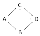
Subpaths include: ABD, AD, ABCD, ACD

Usage

data(simulated)

Format

A list of matrices having 200 rows and 10 variables:

A

Simulated matrix A

B

Simulated matrix B

...

References

Tormod Næs, Rosaria Romano, Oliver Tomic, Ingrid Måge, Age Smilde, Kristian Hovde Liland, Sequential and orthogonalized PLS (SO-PLS) regression for path analysis: Order of blocks and relations between effects. Journal of Chemometrics, In Press

Sparse Multiblock Partial Least Squares - sMB-PLS

Description

sMB-PLS is an adaptation of MB-PLS (mbpls) that enforces sparseness in loading weights when computing PLS components in the global model.

Usage

smbpls(
  formula,
  data,
  subset,
  na.action,
  X = NULL,
  Y = NULL,
  ncomp = 1,
  scale = FALSE,
  shrink = NULL,
  truncation = NULL,
  trunc.width = 0.95,
  blockScale = c("sqrtnvar", "ssq", "none"),
  ...
)

Arguments

Details

Two versions of sparseness are supplied: Soft-Threshold PLS, also known as Sparse PLS, and Truncation PLS. The former uses L1 shrinkage of loading weights, while the latter comes in two flavours, both estimating inliers and outliers. The "Lenth" method uses asymmetric confidence intervals around the median of a loading weigh vector to estimate inliers. The "quantile" method uses a quantile plot approach to estimate outliers as deviations from the estimated quantile line. As with ordinary MB-PLS scaled input blocks (1/sqrt(ncol)) are used.

Block weighting is performed after scaling all variables and is by default "sqrtnvar": 1/sqrt(ncol(X[[i]])) in each block. Alternatives are "ssq": 1/norm(X[[i]], "F")^2 and "none": 1/1. Finally, if a numeric vector is supplied, it will be used to scale the blocks after "ssq" scaling, i.e., Z[[i]] = X[[i]] / norm(X[[i]], "F")^2 * blockScale[i].

Value

multiblock, mvr object with super-scores, super-loadings, block-scores and block-loading, and the underlying mvr (PLS) object for the super model, with all its result and plot possibilities. Relevant plotting functions: multiblock_plots and result functions: multiblock_results.

References

• Sæbø, S.; Almøy, T.; Aarøe, J. & Aastveit, A. ST-PLS: a multi-directional nearest shrunken centroid type classifier via PLS Journal of Chemometrics: A Journal of the Chemometrics Society, Wiley Online Library, 2008, 22, 54-62.

• Lê Cao, K.; Rossouw, D.; Robert-Granié, C. & Besse, P. A sparse PLS for variable selection when integrating omics data Statistical applications in genetics and molecular biology, 2008, 7.

• Liland, K.; Høy, M.; Martens, H. & Sæbø, S. Distribution based truncation for variable selection in subspace methods for multivariate regression Chemometrics and Intelligent Laboratory Systems, 2013, 122, 103-111.

• Karaman, I.; Nørskov, N.; Yde, C.; Hedemann, M.; Knudsen, K. & Kohler, A. Sparse multi-block PLSR for biomarker discovery when integrating data from LC–MS and NMR metabolomics Metabolomics, 2015, 11, 367-379.

See Also

Overviews of available methods, multiblock, and methods organised by main structure: basic, unsupervised, asca, supervised and complex.

Examples

data(potato)

# Truncation MB-PLS 
# Loading weights inside 60% confidence intervals around the median are set to 0.
tmb <- smbpls(Sensory ~ Chemical+Compression, data=potato, ncomp = 5, 
              truncation = "Lenth", trunc.width = 0.6)
              
# Alternative XY-interface
tmb.XY <- smbpls(X=potato[c('Chemical','Compression')], Y=potato[['Sensory']], ncomp = 5, 
              truncation = "Lenth", trunc.width = 0.6)
identical(tmb, tmb.XY)
scoreplot(tmb, labels="names") # Exploiting mvr object structure from pls package
loadingweightplot(tmb, labels="names")

# Soft-Threshold / Sparse MB-PLS 
# Loading weights are subtracted by 60% of maximum value.
smb <- smbpls(X=potato[c('Chemical','Compression')], Y=potato[['Sensory']], 
              ncomp = 5, shrink = 0.6)
print(smb)
scoreplot(smb, labels="names") # Exploiting mvr object structure from pls package
loadingweightplot(smb, labels="names")

# Emphasis may be different for blocks
smb <- smbpls(X=potato[c('Chemical','Compression')], Y=potato[['Sensory']], 
              ncomp = 5, shrink = 0.6, blockScale = c(1, 10))

Sequential and Orthogonalized PLS (SO-PLS)

Description

Function for computing standard SO-PLS based on the interface of the pls package.

Usage

sopls(
  formula,
  ncomp,
  max_comps = min(sum(ncomp), 20),
  data,
  subset,
  na.action,
  scale = FALSE,
  validation = c("none", "CV", "LOO"),
  sequential = FALSE,
  segments = 10,
  sel.comp = "opt",
  progress = TRUE,
  ...
)

Arguments

Details

SO-PLS is a method which handles two or more input blocks by sequentially performing PLS on blocks against a response and orthogonalising the remaining blocks on the extracted components. Component number optimisation can either be done globally (best combination across blocks) or sequentially (determine for one block, move to next, etc.).

Value

An sopls, mvr object with scores, loadings, etc. associated with printing (sopls_results) and plotting methods (sopls_plots).

References

Jørgensen K, Mevik BH, Næs T. Combining designed experiments with several blocks of spectroscopic data. Chemometr Intell Lab Syst. 2007;88(2): 154–166.

See Also

SO-PLS result functions, sopls_results, SO-PLS plotting functions, sopls_plots, SO-PLS Måge plot, maage, and SO-PLS path-modelling, SO_TDI. Overviews of available methods, multiblock, and methods organised by main structure: basic, unsupervised, asca, supervised and complex.

Examples

data(potato)
so <- sopls(Sensory ~ Chemical + Compression, data=potato, ncomp=c(10,10), 
            max_comps=10, validation="CV", segments=10)
summary(so)

# Scatter plot matrix with two first components from Chemical block
# and 1 component from the Compression block.
scoreplot(so, comps=list(1:2,1), ncomp=2, block=2)

# Result functions and more plots for SO-PLS 
# are found in ?sopls_results and ?sopls_plots.

Scores, loadings and plots for sopls objects

Description

Extraction of scores and loadings and adaptation of scoreplot, loadingplot and biplot from package pls for sopls objects.

Usage

## S3 method for class 'sopls'
loadings(object, ncomp = "all", block = 1, y = FALSE, ...)

## S3 method for class 'sopls'
scores(object, ncomp = "all", block = 1, y = FALSE, ...)

## S3 method for class 'sopls'
scoreplot(
  object,
  comps = 1:2,
  ncomp = NULL,
  block = 1,
  labels,
  identify = FALSE,
  type = "p",
  xlab,
  ylab,
  ...
)

## S3 method for class 'sopls'
loadingplot(
  object,
  comps = 1:2,
  ncomp = NULL,
  block = 1,
  scatter = TRUE,
  labels,
  identify = FALSE,
  type,
  lty,
  lwd = NULL,
  pch,
  cex = NULL,
  col,
  legendpos,
  xlab,
  ylab,
  pretty.xlabels = TRUE,
  xlim,
  ...
)

## S3 method for class 'sopls'
corrplot(
  object,
  comps = 1:2,
  ncomp = NULL,
  block = 1,
  labels = TRUE,
  col = 1:5,
  plotx = TRUE,
  ploty = TRUE,
  ...
)

## S3 method for class 'sopls'
biplot(
  x,
  comps = 1:2,
  ncomp = "all",
  block = 1,
  which = c("x", "y", "scores", "loadings"),
  var.axes = FALSE,
  xlabs,
  ylabs,
  main,
  ...
)

Arguments

Details

If comps is supplied as a list for scoreplot, it is assumed that its elements refer to each of the blocks up to block number block. For instance comps = list(1, 0, 1:2) will select 1 component from the first block, no components from the second block and the first two components from the last block. This must be matched by ncomp, specifying how many components were selected before block number block.

See Also

Overviews of available methods, multiblock, and methods organised by main structure: basic, unsupervised, asca, supervised and complex. Common functions for computation and extraction of results are found in sopls_results.

#' @return The score and loading functions return scores and loadings, while plot functions have no return (except use of 'identify').

Examples

data(potato)
so <- sopls(Sensory ~ Chemical + Compression + NIRraw, data=potato, ncomp=c(5,5,5))

# Loadings
loadings(so, ncomp=c(3), block=2)[, 1:3]

# Scores
scores(so, block=1)[, 1:4]

# Default plot from first block
scoreplot(so)

# Second block with names
scoreplot(so, ncomp=c(3), block=2, labels="names")

# Scatterplot matrix
scoreplot(so, ncomp=c(3,2), block=3, comps=1:3)

# Combination of blocks (see Details)
scoreplot(so, ncomp=c(3,2), block=3, comps=list(1,0,1))

# Default plot from first block
loadingplot(so, scatter=TRUE)

# Second block with names
loadingplot(so, ncomp=c(3), block=2, labels="names", scatter=TRUE)

# Scatterplot matrix
loadingplot(so, ncomp=c(3,2), block=3, comps=1:3, scatter=TRUE)

# Correlation loadings
corrplot(so, block=2, ncomp=1)

# Default plot from first block
biplot(so)

Result functions for SO-PLS models

Description

Standard result functions for SO-PLS (sopls).

Usage

## S3 method for class 'sopls'
predict(
  object,
  newdata,
  ncomp = object$ncomp,
  type = c("response", "scores"),
  na.action = na.pass,
  ...
)

## S3 method for class 'sopls'
coef(object, ncomp = object$ncomp, intercept = FALSE, ...)

## S3 method for class 'sopls'
print(x, ...)

## S3 method for class 'sopls'
summary(
  object,
  what = c("all", "validation", "training"),
  digits = 4,
  print.gap = 2,
  ...
)

classify(object, ...)

## S3 method for class 'sopls'
classify(object, classes, newdata, ncomp, LQ = "LDA", ...)

## S3 method for class 'sopls'
R2(object, estimate, newdata, ncomp = "all", individual = FALSE, ...)

## S3 method for class 'sopls'
RMSEP(object, estimate, newdata, ncomp = "all", individual = FALSE, ...)

pcp(object, ...)

## S3 method for class 'sopls'
pcp(object, ncomp, ...)

## Default S3 method:
pcp(object, X, ...)

cvanova(pred, ...)

## Default S3 method:
cvanova(pred, true, absRes = TRUE, ...)

## S3 method for class 'sopls'
cvanova(pred, comps, absRes = TRUE, ...)

## S3 method for class 'cvanova'
print(x, ...)

## S3 method for class 'cvanova'
summary(object, ...)

## S3 method for class 'cvanova'
plot(x, ...)

## S3 method for class 'sopls'
residuals(object, ...)

Arguments

Details

The parameter ncomp controls which components to apply/extract, resulting in the sequence of components leading up to the specific choice, i.e. ncomp = c(2,2,1) results in the sequence 1,0,0; 2,0,0; 2,1,0; 2,2,0; 2,2,1. Usage of the functions are shown using generics in the examples below. Prediction, regression coefficients, object printing and summary are available through: predict.sopls, coef.sopls, print.sopls and summary.sopls. Explained variances and RMSEP are available through R2.sopls and RMSEP.sopls. Principal components of predictions are available through pcp.sopls. Finally, there is work in progress on classifcation support through classify.sopls.

Value

Returns depend on method used, e.g. predict.sopls returns predicted responses or scores depending on inputs, coef.sopls return regression coefficients, while print and summary methods return the object invisibly.

References

Jørgensen K, Mevik BH, Næs T. Combining designed experiments with several blocks of spectroscopic data. Chemometr Intell Lab Syst. 2007;88(2): 154–166.

See Also

Overviews of available methods, multiblock, and methods organised by main structure: basic, unsupervised, asca, supervised and complex. Common functions for plotting are found in sopls_plots.

Examples

data(potato)
mod <- sopls(Sensory[,1] ~ ., data = potato[c(1:3,9)], ncomp = 5, subset = 1:20)
testset <- potato[-(1:20),]; testset$Sensory <- testset$Sensory[,1,drop=FALSE]
predict(mod, testset, ncomp=c(2,1,2))
dim(coef(mod, ncomp=c(3,0,1))) # <variables x responses x components>
R2(mod, ncomp = c(4,1,2))
print(mod)
summary(mod)

# PCP from sopls object
modMulti <- sopls(Sensory ~ ., data = potato[c(1:3,9)], ncomp = 5, validation = "CV", segment = 5)
(PCP <- pcp(modMulti, c(2,1,2)))
scoreplot(PCP)

# PCP from matrices
preds <- modMulti$validation$Ypred[,,"2,1,2"]
PCP_default <- pcp(preds, potato[1:3])

# CVANOVA
modCV <- sopls(Sensory[,1] ~ ., data = potato[c(1:3,9)], ncomp = 5, validation = "CV", segment = 5)
summary(cva <- cvanova(modCV, "2,1,2"))
plot(cva)

Structuration des Tableaux à Trois Indices de la Statistique - STATIS

Description

This is a wrapper for the ade4::statis function for computing STATIS.

Usage

statis(X, ncomp = 3, scannf = FALSE, tol = 1e-07, ...)

Arguments

Details

STATIS is a method, related to MFA, for analysing two or more blocks. It also decomposes the data into a low-dimensional subspace but uses a different scaling of the individual blocks.

Value

multiblock object including relevant scores and loadings. Relevant plotting functions: multiblock_plots and result functions: multiblock_results.

References

Lavit, C.; Escoufier, Y.; Sabatier, R.; Traissac, P. (1994). The ACT (STATIS method). Computational Statistics & Data Analysis. 18: 97

See Also

Overviews of available methods, multiblock, and methods organised by main structure: basic, unsupervised, asca, supervised and complex. Common functions for computation and extraction of results and plotting are found in multiblock_results and multiblock_plots, respectively.

Examples

data(candies)
candyList <- lapply(1:nlevels(candies$candy),function(x)candies$assessment[candies$candy==x,])
can.statis <- statis(candyList)
plot(scores(can.statis), labels="names")

Supervised Multiblock Methods

Description

Collection of supervised multiblock methods:

• MB-PLS - Multiblock Partial Least Squares (mbpls)

• sMB-PLS - Sparse Multiblock Partial Least Squares (smbpls)

• SO-PLS - Sequential and Orthogonalized PLS (sopls)

• PO-PLS - Parallel and Orthogonalized PLS (popls)

• ROSA - Response Oriented Sequential Alternation (rosa)

• mbRDA - Multiblock Redundancy Analysis (mbrda)

See Also

Overviews of available methods, multiblock, and methods organised by main structure: basic, unsupervised, asca, supervised and complex. Common functions for computation and extraction of results and plotting are found in multiblock_results and multiblock_plots, respectively.

Examples

data(potato)
mb <- mbpls(Sensory ~ Chemical + Compression, data=potato, ncomp = 5)
print(mb)

# Convert data.frame with AsIs objects to list of matrices
potatoList <- lapply(potato, unclass)
mbr <- mbrda(Sensory ~ Chemical + Compression, data=potatoList, ncomp = 10)
print(mbr)
scoreplot(mbr, labels="names")

Unique combinations of blocks

Description

Compute a list of all possible block combinations where the number of blocks in each combination is limited by parameters min_level and max_level.

Usage

unique_combos(n_block, max_level, min_level = 2)

Arguments

Details

This function is used for minimal redundancy implementations of rosa and sopls and for lookups into computed components.

Value

A list of unique block combinations.

Examples

unique_combos(3, 2)

Unsupervised Multiblock Methods

Description

Collection of unsupervised multiblock methods:

• SCA - Simultaneous Component Analysis (sca)

• GCA - Generalized Canonical Analysis (gca)

• GPA - Generalized Procrustes Analysis (gpa)

• MFA - Multiple Factor Analysis (mfa)

• PCA-GCA (pcagca)

• DISCO - Distinctive and Common Components with SCA (disco)

• HPCA - Hierarchical Principal component analysis (hpca)

• MCOA - Multiple Co-Inertia Analysis (mcoa)

• JIVE - Joint and Individual Variation Explained (jive)

• STATIS - Structuration des Tableaux à Trois Indices de la Statistique (statis)

• HOGSVD - Higher Order Generalized SVD (hogsvd)

Details

Original documentation of STATIS: statis. JIVE, STATIS and HOGSVD assume variable linked matrices/data.frames, while SCA handles both links.

See Also

Overviews of available methods, multiblock, and methods organised by main structure: basic, unsupervised, asca, supervised and complex. Common functions for computation and extraction of results and plotting are found in multiblock_results and multiblock_plots, respectively.

Examples

# Object linked data
data(potato)
potList <- as.list(potato[c(1,2,9)])
pot.sca    <- sca(potList)

# Variable linked data
data(candies)
candyList <- lapply(1:nlevels(candies$candy),function(x)candies$assessment[candies$candy==x,])
can.statis <- statis(candyList)
plot(can.statis$statis)

Wines of Val de Loire

Description

This dataset contains sensory assessment of 21 wines. The assessments are grouped according to the tasting process and thus have a natural ordering with a all blocks pointing forward to all remaining blocks in the process.

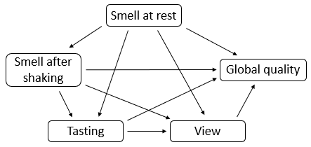
Usage

data(wine)

Format

A data.frame having 21 rows and 5 variables:

Smell at rest

Matrix of sensory assessments

View

Matrix of sensory assessments

Smell after shaking

Matrix of sensory assessments

Tasting

Matrix of sensory assessments

Global quality

Matrix of sensory assessments

References

Escofier B, Pages L. Analyses Factorielles Simples and Multiples. Paris: Dunod; 1988.