| Title: | Dynamic Multi-Species Size Spectrum Modelling |
| Date: | 2025-11-16 |
| Type: | Package |
| Description: | A set of classes and methods to set up and run multi-species, trait based and community size spectrum ecological models, focused on the marine environment. |
| Maintainer: | Gustav Delius <gustav.delius@york.ac.uk> |
| Version: | 2.5.4 |
| License: | GPL-3 |
| Imports: | assertthat, deSolve, dplyr, ggplot2 (≥ 3.4.0), ggrepel, grid, lubridate, methods, plotly, plyr, progress, Rcpp, reshape2, rlang, lifecycle |
| LinkingTo: | Rcpp |
| Depends: | R (≥ 3.1) |
| Suggests: | testthat (≥ 3.0.0), vdiffr, diffviewer, roxygen2, knitr, rmarkdown, pkgdown, covr, spelling |
| Collate: | 'age_mat.R' 'helpers.R' 'MizerParams-class.R' 'MizerSim-class.R' 'reproduction.R' 'saveParams.R' 'species_params.R' 'setColours.R' 'setInteraction.R' 'setPredKernel.R' 'setSearchVolume.R' 'setMaxIntakeRate.R' 'setMetabolicRate.R' 'setMetadata.R' 'setExtMort.R' 'setExtEncounter.R' 'setReproduction.R' 'setResource.R' 'setFishing.R' 'setInitialValues.R' 'setBevertonHolt.R' 'upgrade.R' 'selectivity_funcs.R' 'pred_kernel_funcs.R' 'resource_dynamics.R' 'resource_semichemostat.R' 'resource_logistic.R' 'project.R' 'mizer-package.R' 'project_methods.R' 'rate_functions.R' 'summary_methods.R' 'plots.R' 'plotBiomassObservedVsModel.R' 'plotYieldObservedVsModel.R' 'animateSpectra.R' 'newMultispeciesParams.R' 'wrapper_functions.R' 'newSingleSpeciesParams.R' 'steady.R' 'extension.R' 'data.R' 'RcppExports.R' 'deprecated.R' 'get_initial_n.R' 'compareParams.R' 'customFunction.R' 'manipulate_species.R' 'calibrate.R' 'match.R' 'matchGrowth.R' 'steadySingleSpecies.R' 'defaults_edition.R' 'validSpeciesParams.R' |
| RoxygenNote: | 7.3.3 |
| Encoding: | UTF-8 |
| LazyData: | true |
| URL: | https://sizespectrum.org/mizer/, https://github.com/sizespectrum/mizer |
| BugReports: | https://github.com/sizespectrum/mizer/issues |
| Language: | en-GB |
| RdMacros: | lifecycle |
| VignetteBuilder: | knitr |
| Config/testthat/edition: | 3 |
| NeedsCompilation: | yes |
| Packaged: | 2025-11-16 21:31:14 UTC; gustav |
| Author: | Gustav Delius  [cre, aut, cph],
Finlay Scott [aut, cph],
Julia Blanchard
[aut, cph],
Ken Andersen
[aut, cph],
Richard Southwell [ctb, cph]
[cre, aut, cph],
Finlay Scott [aut, cph],
Julia Blanchard
[aut, cph],
Ken Andersen
[aut, cph],
Richard Southwell [ctb, cph] |
| Repository: | CRAN |
| Date/Publication: | 2025-11-16 21:50:02 UTC |
mizer: Multi-species size-based modelling in R
Description
The mizer package implements multi-species size-based modelling in R. It has been designed for modelling marine ecosystems.
Details
Using mizer is relatively simple. There are three main stages:
-
Setting the model parameters. This is done by creating an object of class MizerParams. This includes model parameters such as the life history parameters of each species, and the range of the size spectrum. There are several setup functions that help to create a MizerParams objects for particular types of models:
-
Running a simulation. This is done by calling the
project()function with the model parameters. This produces an object of MizerSim that contains the results of the simulation. -
Exploring results. After a simulation has been run, the results can be explored using a range of plotting_functions, summary_functions and indicator_functions.
See the mizer website for full details of the principles behind mizer and how the package can be used to perform size-based modelling.
Author(s)
Maintainer: Gustav Delius gustav.delius@york.ac.uk (ORCID) [copyright holder]
Authors:
Finlay Scott drfinlayscott@gmail.com [copyright holder]
Julia Blanchard julia.blanchard@utas.edu.au (ORCID) [copyright holder]
Ken Andersen kha@aqua.dtu.dk (ORCID) [copyright holder]
Other contributors:
Richard Southwell richard.southwell@york.ac.uk [contributor, copyright holder]
See Also
Useful links:
Report bugs at https://github.com/sizespectrum/mizer/issues
Beverton Holt function to calculate density-dependent reproduction rate
Description
Takes the density-independent rates R_{di} of egg production (as
calculated by getRDI()) and returns
reduced, density-dependent reproduction rates R_{dd} given as
R_{dd} = R_{di}
\frac{R_{max}}{R_{di} + R_{max}}
where
R_{max} are the maximum possible reproduction rates that must be
specified in a column in the species parameter dataframe.
(All quantities in the above equation are species-specific but we dropped
the species index for simplicity.)
Usage
BevertonHoltRDD(rdi, species_params, ...)
Arguments
rdi |
Vector of density-independent reproduction rates
|
species_params |
A species parameter dataframe. Must contain a column
|
... |
Unused |
Details
This is only one example of a density-dependence. You can write your own
function based on this example, returning different density-dependent
reproduction rates. Three other examples provided are RickerRDD(),
SheperdRDD(), noRDD() and constantRDD(). For more explanation see
setReproduction().
Value
Vector of density-dependent reproduction rates.
See Also
Other functions calculating density-dependent reproduction rate:
RickerRDD(),
SheperdRDD(),
constantEggRDI(),
constantRDD(),
noRDD()
Alias for set_multispecies_model()
Description
![[Deprecated]](./figures/lifecycle-deprecated.svg) An alias provided for backward compatibility with mizer version <= 1.0
An alias provided for backward compatibility with mizer version <= 1.0
Usage
MizerParams(
  species_params,
  interaction = matrix(1, nrow = nrow(species_params), ncol = nrow(species_params)),
  min_w_pp = 1e-10,
  min_w = 0.001,
  max_w = NULL,
  no_w = 100,
  n = 2/3,
  q = 0.8,
  f0 = 0.6,
  kappa = 1e+11,
  lambda = 2 + q - n,
  r_pp = 10,
  ...
)
Arguments
species_params |
A data frame of species-specific parameter values. |
interaction |
Optional interaction matrix of the species (predator species x prey species). By default all entries are 1. See "Setting interaction matrix" section below. |
min_w_pp |
The smallest size of the resource spectrum. By default this is set to the smallest value at which any of the consumers can feed. |
min_w |
Sets the size of the eggs of all species for which this is not
given in the |
max_w |
The largest size of the consumer spectrum. By default this is
set to the largest |
no_w |
The number of size bins in the consumer spectrum. |
n |
The allometric growth exponent. This can be overruled for individual
species by including a |
q |
Allometric exponent of search volume |
f0 |
Expected average feeding level. Used to set |
kappa |
The coefficient of the initial resource abundance power-law. |
lambda |
Used to set power-law exponent for resource capacity if the
|
r_pp |
|
... |
Unused |
Value
A MizerParams object
A class to hold the parameters for a size based model.
Description
Although it is possible to build a MizerParams object by hand it is
not recommended and several constructors are available. Dynamic simulations
are performed using project() function on objects of this class. As a
user you should never need to access the slots inside a MizerParams object
directly.
Details
The MizerParams class is fairly complex with a large number of
slots, many of which are multidimensional arrays. The dimensions of these
arrays is strictly enforced so that MizerParams objects are consistent
in terms of number of species and number of size classes.
The MizerParams class does not hold any dynamic information, e.g.
abundances or harvest effort through time. These are held in
MizerSim objects.
Slots
metadataA list with metadata information. See
setMetadata().mizer_versionThe package version of mizer (as returned by
packageVersion("mizer")) that created or upgraded the model.extensionsA named vector of strings where each name is the name of and extension package needed to run the model and each value is a string giving the information that the remotes package needs to install the correct version of the extension package, see https://remotes.r-lib.org/.
time_createdA POSIXct date-time object with the creation time.
time_modifiedA POSIXct date-time object with the last modified time.
wThe size grid for the fish part of the spectrum. An increasing vector of weights (in grams) running from the smallest egg size to the largest maximum size.
dwThe widths (in grams) of the size bins
w_fullThe size grid for the full size range including the resource spectrum. An increasing vector of weights (in grams) running from the smallest resource size to the largest maximum size of fish. The last entries of the vector have to be equal to the content of the w slot.
dw_fullThe width of the size bins for the full spectrum. The last entries have to be equal to the content of the dw slot.
w_min_idxA vector holding the index of the weight of the egg size of each species
maturityAn array (species x size) that holds the proportion of individuals of each species at size that are mature. This enters in the calculation of the spawning stock biomass with
getSSB(). Set withsetReproduction().psiAn array (species x size) that holds the allocation to reproduction for each species at size,
\psi_i(w). Changed withsetReproduction().intake_maxAn array (species x size) that holds the maximum intake for each species at size. Changed with
setMaxIntakeRate().search_volAn array (species x size) that holds the search volume for each species at size. Changed with
setSearchVolume().metabAn array (species x size) that holds the metabolism for each species at size. Changed with
setMetabolicRate().mu_bAn array (species x size) that holds the external mortality rate
\mu_{ext.i}(w). Changed withsetExtMort().ext_encounterAn array (species x size) that holds the external encounter rate
E_{ext.i}(w). Changed withsetExtEncounter().pred_kernelAn array (species x predator size x prey size) that holds the predation coefficient of each predator at size on each prey size. If this is NA then the following two slots will be used. Changed with
setPredKernel().ft_pred_kernel_eAn array (species x log of predator/prey size ratio) that holds the Fourier transform of the feeding kernel in a form appropriate for evaluating the encounter rate integral. If this is NA then the
pred_kernelwill be used to calculate the available energy integral. Changed withsetPredKernel().ft_pred_kernel_pAn array (species x log of predator/prey size ratio) that holds the Fourier transform of the feeding kernel in a form appropriate for evaluating the predation mortality integral. If this is NA then the
pred_kernelwill be used to calculate the integral. Changed withsetPredKernel().rr_ppA vector the same length as the w_full slot. The size specific growth rate of the resource spectrum.
cc_ppA vector the same length as the w_full slot. The size specific carrying capacity of the resource spectrum.
resource_dynamicsName of the function for projecting the resource abundance density by one timestep.
other_dynamicsA named list of functions for projecting the values of other dynamical components of the ecosystem that may be modelled by a mizer extensions you have installed. The names of the list entries are the names of those components.
other_encounterA named list of functions for calculating the contribution to the encounter rate from each other dynamical component.
other_mortA named list of functions for calculating the contribution to the mortality rate from each other dynamical components.
other_paramsA list containing the parameters needed by any mizer extensions you may have installed to model other dynamical components of the ecosystem.
rates_funcsA named list with the names of the functions that should be used to calculate the rates needed by
project(). By default this will be set to the names of the built-in rate functions.sc![[Experimental]](./figures/lifecycle-experimental.svg) The community abundance of the scaling community
The community abundance of the scaling communityspecies_paramsA data.frame to hold the species specific parameters. See
species_params()for details.given_species_paramsA data.frame to hold the species parameters that were given explicitly rather than obtained by default calculations.
gear_paramsData frame with parameters for gear selectivity. See
setFishing()for details.interactionThe species specific interaction matrix,
\theta_{ij}. Changed withsetInteraction().selectivityAn array (gear x species x w) that holds the selectivity of each gear for species and size,
S_{g,i,w}. Changed withsetFishing().catchabilityAn array (gear x species) that holds the catchability of each species by each gear,
Q_{g,i}. Changed withsetFishing().initial_effortA vector containing the initial fishing effort for each gear. Changed with
setFishing().initial_nAn array (species x size) that holds the initial abundance of each species at each weight.
initial_n_ppA vector the same length as the w_full slot that describes the initial resource abundance at each weight.
initial_n_otherA list with the initial abundances of all other ecosystem components. Has length zero if there are no other components.
resource_paramsList with parameters for resource.
A-
Abundance multipliers.
linecolourA named vector of colour values, named by species. Used to give consistent colours in plots.
linetypeA named vector of linetypes, named by species. Used to give consistent line types in plots.
ft_maskAn array (species x w_full) with zeros for weights larger than the maximum weight of each species. Used to efficiently minimize wrap-around errors in Fourier transform calculations.
See Also
project() MizerSim()
emptyParams() newMultispeciesParams()
newCommunityParams()
newTraitParams()
Constructor for the MizerSim class
Description
A constructor for the MizerSim class. This is used by
project() to create MizerSim objects of the right
dimensions. It is not necessary for users to use this constructor.
Usage
MizerSim(params, t_dimnames = NA, t_max = 100, t_save = 1)
Arguments
params |
a MizerParams object |
t_dimnames |
Numeric vector that is used for the time dimensions of the slots. Default = NA. |
t_max |
The maximum time step of the simulation. Only used if t_dimnames = NA. Default value = 100. |
t_save |
How often should the results of the simulation be stored. Only used if t_dimnames = NA. Default value = 1. |
Value
An object of type MizerSim
A class to hold the results of a simulation
Description
A class that holds the results of projecting a MizerParams
object through time using project().
Details
A new MizerSim object can be created with the MizerSim()
constructor, but you will never have to do that because the object is
created automatically by project() when needed.
As a user you should never have to access the slots of a MizerSim object
directly. Instead there are a range of functions to extract the information.
N() and NResource() return arrays with the saved abundances of
the species and the resource population at size respectively. getEffort()
returns the fishing effort of each gear through time.
getTimes() returns the vector of times at which simulation results
were stored and idxFinalT() returns the index with which to access
specifically the value at the final time in the arrays returned by the other
functions. getParams() returns the MizerParams object that was
passed to project(). There are also several
summary_functions and plotting_functions
available to explore the contents of a MizerSim object.
The arrays all have named dimensions. The names of the time dimension
denote the time in years. The names of the w dimension are weights in grams
rounded to three significant figures. The names of the sp dimension are the
same as the species name in the order specified in the species_params data
frame. The names of the gear dimension are the names of the gears, in the
same order as specified when setting up the MizerParams object.
Extensions of mizer can use the n_other slot to store the abundances of
other ecosystem components and these extensions should provide their own
functions for accessing that information.
The MizerSim class has changed since previous versions of mizer. To use
a MizerSim object created by a previous version, you need to upgrade it
with upgradeSim().
Slots
paramsAn object of type MizerParams.
nThree-dimensional array (time x species x size) that stores the projected community number densities.
n_ppAn array (time x size) that stores the projected resource number densities.
n_otherA list array (time x component) that stores the projected values for other ecosystem components.
effortAn array (time x gear) that stores the fishing effort by time and gear.
Time series of size spectra
Description
Fetch the simulation results for the size spectra over time.
Usage
N(sim)

NResource(sim)
Arguments
sim |
A MizerSim object |
Value
For N(): A three-dimensional array (time x species x size) with the
number density of consumers
For NResource(): An array (time x size) with the number density of resource
Examples
str(N(NS_sim))
str(NResource(NS_sim))
Time series of other components
Description
Fetch the simulation results for other components over time.
Usage
NOther(sim)
Arguments
sim |
A MizerSim object |
Value
A list array (time x component) that stores the projected values for other ecosystem components.
Example interaction matrix for the North Sea example
Description
The interaction coefficient between predator and prey species in the North Sea.
Usage
NS_interaction
Format
A 12 x 12 matrix.
Source
Blanchard et al.
Examples
params <- MizerParams(NS_species_params_gears,
                      interaction = NS_interaction)
Example MizerParams object for the North Sea example
Description
A MizerParams object created from the NS_species_params_gears species
parameters and the inter interaction matrix together with an initial
condition corresponding to the steady state obtained from fishing with an
effort
effort = c(Industrial = 0, Pelagic = 1, Beam = 0.5, Otter = 0.5).
Usage
NS_params
Format
A MizerParams object
Source
Blanchard et al.
See Also
Other example parameter objects:
NS_sim
Examples
sim = project(NS_params, effort = c(Industrial = 0, Pelagic = 1,
                                    Beam = 0.5, Otter = 0.5))
plot(sim)
Example MizerSim object for the North Sea example
Description
A MizerSim object containing a simulation with historical fishing mortalities from the North Sea, as created in the tutorial "A Multi-Species Model of the North Sea".
Usage
NS_sim
Format
A MizerSim object
Source
https://sizespectrum.org/mizer/articles/a_multispecies_model_of_the_north_sea.html
See Also
Other example parameter objects:
NS_params
Examples
plotBiomass(NS_sim)
Example species parameter set based on the North Sea
Description
This data set is based on species in the North Sea (Blanchard et al.). It is
a data.frame that contains all the necessary information to be used by the
MizerParams() constructor. As there is no gear column, each species is
assumed to be fished by a separate gear.
Usage
NS_species_params
Format
A data frame with 12 rows and 7 columns. Each row is a species.
- species
Name of the species
- w_max
Maximum size.
- w_mat
Size at maturity
- beta
Size preference ratio
- sigma
Width of the size-preference
- R_max
Maximum reproduction rate
- k_vb
The von Bertalanffy k parameter
- w_inf
The von Bertalanffy asymptotic size
Source
Blanchard et al.
Examples
params <- MizerParams(NS_species_params)
Example species parameter set based on the North Sea with different gears
Description
This data set is based on species in the North Sea (Blanchard et al.).
It is similar to the data set NS_species_params except that
this one has an additional column specifying the fishing gear that
operates on each species.
Usage
NS_species_params_gears
Format
A data frame with 12 rows and 8 columns. Each row is a species.
- species
Name of the species
- w_max
Maximum size.
- w_mat
Size at maturity
- beta
Size preference ratio
- sigma
Width of the size-preference
- R_max
Maximum reproduction rate
- k_vb
The von Bertalanffy k parameter
- w_inf
The von Bertalanffy asymptotic size
- gear
Name of the fishing gear
Source
Blanchard et al.
Examples
params <- MizerParams(NS_species_params_gears)
Ricker function to calculate density-dependent reproduction rate
Description
Takes the density-independent rates R_{di} of egg production and
returns reduced, density-dependent rates R_{dd} given as
R_{dd} = R_{di} \exp(- b R_{di})
Usage
RickerRDD(rdi, species_params, ...)
Arguments
rdi |
Vector of density-independent reproduction rates
|
species_params |
A species parameter dataframe. Must contain a column
|
... |
Unused |
Value
Vector of density-dependent reproduction rates.
See Also
Other functions calculating density-dependent reproduction rate:
BevertonHoltRDD(),
SheperdRDD(),
constantEggRDI(),
constantRDD(),
noRDD()
Sheperd function to calculate density-dependent reproduction rate
Description
Takes the density-independent rates R_{di} of egg production and returns
reduced, density-dependent rates R_{dd} given as
R_{dd} = \frac{R_{di}}{1+(b\ R_{di})^c}
Usage
SheperdRDD(rdi, species_params, ...)
Arguments
rdi |
Vector of density-independent reproduction rates
|
species_params |
A species parameter dataframe. Must contain columns
|
... |
Unused |
Details
With b = 1/R_{max} and c = 1 this reduces to the Beverton-Holt
reproduction rate, see BevertonHoltRDD().
Value
Vector of density-dependent reproduction rates.
See Also
Other functions calculating density-dependent reproduction rate:
BevertonHoltRDD(),
RickerRDD(),
constantEggRDI(),
constantRDD(),
noRDD()
Add new species
Description
Takes a MizerParams object and adds additional species with given parameters to the ecosystem. It sets the initial values for these new species to their steady-state solution in the given initial state of the existing ecosystem. This will be close to the true steady state if the abundances of the new species are sufficiently low. Hence the abundances of the new species are set so that they are at most 1/100th of the resource power law. Their reproductive efficiencies are set so as to keep them at that low level.
Usage
addSpecies(
  params,
  species_params,
  gear_params = data.frame(),
  initial_effort,
  interaction
)
Arguments
params |
A mizer params object for the original system. |
species_params |
Data frame with the species parameters of the new species we want to add to the system. |
gear_params |
Data frame with the gear parameters for the new species. If not provided then the new species will not be fished. |
initial_effort |
A named vector with the effort for any new fishing gear
introduced in |
interaction |
Interaction matrix. A square matrix giving either the interaction coefficients between all species or only those between the new species. In the latter case all interaction between an old and a new species are set to 1. If this argument is missing, all interactions involving a new species are set to 1. |
Details
The resulting MizerParams object will use the same size grid where possible, but if one of the new species needs a larger range of w (either because a new species has an egg size smaller than those of existing species or a maximum size larger than those of existing species) then the grid will be expanded and all arrays will be enlarged accordingly.
If any of the rate arrays of the existing species had been set by the user to values other than those calculated as default from the species parameters, then these will be preserved. Only the rates for the new species will be calculated from their species parameters.
After adding the new species, the background species are not retuned and
the system is not run to steady state. This could be done with steady().
The new species will have a reproduction level of 1/4, this can then be
changed with setBevertonHolt()
Value
An object of type MizerParams
See Also
Examples
params <- newTraitParams()
species_params <- data.frame(
    species = "Mullet",
    w_max = 173,
    w_mat = 15,
    beta = 283,
    sigma = 1.8,
    h = 30,
    a = 0.0085,
    b = 3.11
)
params <- addSpecies(params, species_params)
plotSpectra(params)
Calculate age at maturity
Description
Uses the growth rate and the size at maturity to calculate the age at maturity
Usage
age_mat(params)
Arguments
params |
A MizerParams object |
Details
Using that by definition of the growth rate g(w) = dw/dt we have that
\mathrm{age_{mat}} = \int_0^{w_{mat}.}\frac{dw}{g(w)}
Value
A named vector. The names are the species names and the values are the ages at maturity.
Examples
age_mat(NS_params)
Calculate age at maturity from von Bertalanffy growth parameters
Description
This is not a good way to determine the age at maturity because the von Bertalanffy growth curve is not reliable for larvae and juveniles. However this was used in previous versions of mizer and is supplied for backwards compatibility.
Usage
age_mat_vB(object)
Arguments
object |
A MizerParams object or a species_params data frame |
Details
Uses the age at maturity that is implied by the von Bertalanffy growth curve
specified by the w_inf, k_vb, t0, a and b parameters in the
species_params data frame.
If any of k_vb is missing for a species, the function returns NA for that
species. Default values of b = 3 and t0 = 0 are used if these are
missing. If w_inf is missing, w_max is used instead.
Value
A named vector. The names are the species names and the values are the ages at maturity.
Animation of the abundance spectra
Description
Usage
animateSpectra(
  sim,
  species = NULL,
  time_range,
  wlim = c(NA, NA),
  ylim = c(NA, NA),
  power = 1,
  total = FALSE,
  resource = TRUE
)
Arguments
sim |
A MizerSim object |
species |
Name or vector of names of the species to be plotted. By default all species are plotted. |
time_range |
The time range to animate over. Either a vector of values or a vector of min and max time. Default is the entire time range of the simulation. |
wlim |
A numeric vector of length two providing lower and upper limits for the w axis. Use NA to refer to the existing minimum or maximum. |
ylim |
A numeric vector of length two providing lower and upper limits for the y axis. Use NA to refer to the existing minimum or maximum. Any values below 1e-20 are always cut off. |
power |
The abundance is plotted as the number density times the weight
raised to |
total |
A boolean value that determines whether the total over all species in the system is plotted as well. Default is FALSE. |
resource |
A boolean value that determines whether resource is included. Default is TRUE. |
Value
A plotly object
See Also
Other plotting functions:
plot,MizerParams,missing-method,
plot,MizerSim,missing-method,
plotBiomass(),
plotDiet(),
plotFMort(),
plotFeedingLevel(),
plotGrowthCurves(),
plotPredMort(),
plotSpectra(),
plotYield(),
plotYieldGear(),
plotting_functions
Examples
animateSpectra(NS_sim, power = 2, wlim = c(0.1, NA), time_range = 1997:2007)
Box predation kernel
Description
A predation kernel where the predator/prey mass ratio is uniformly distributed on an interval.
Usage
box_pred_kernel(ppmr, ppmr_min, ppmr_max)
Arguments
ppmr |
A vector of predator/prey size ratios |
ppmr_min |
Minimum predator/prey mass ratio |
ppmr_max |
Maximum predator/prey mass ratio |
Details
Writing the predator mass as w and the prey mass as w_p, the
feeding kernel is 1 if w/w_p is between ppmr_min and
ppmr_max and zero otherwise. The parameters need to be given in the
species parameter dataframe in the columns ppmr_min and
ppmr_max.
Value
A vector giving the value of the predation kernel at each of the
predator/prey mass ratios in the ppmr argument.
See Also
Other predation kernel:
lognormal_pred_kernel(),
power_law_pred_kernel(),
truncated_lognormal_pred_kernel()
Examples
params <- NS_params
# Set all required paramters before changing kernel type
species_params(params)$ppmr_max <- 4000
species_params(params)$ppmr_min <- 200
species_params(params)$pred_kernel_type <- "box"
plot(w_full(params), getPredKernel(params)["Cod", 10, ], type="l", log="x")
Calculate selectivity from gear parameters
Description
This function calculates the selectivity for each gear, species and size from
the gear parameters. It is called by setFishing() when the selectivity is
not set by the user.
Usage
calc_selectivity(params)
Arguments
params |
A MizerParams object |
Value
An array (gear x species x size) with the selectivity values
Examples
params <- NS_params
str(calc_selectivity(params))
calc_selectivity(params)["Pelagic", "Herring", ]
Calibrate the model scale to match total observed biomass
Description
Given a MizerParams object params for which biomass observations are
available for at least some species via the biomass_observed column in the
species_params data frame, this function returns an updated MizerParams
object which is rescaled with scaleModel() so that the total biomass in
the model agrees with the total observed biomass.
Usage
calibrateBiomass(params)
Arguments
params |
A MizerParams object |
Details
Biomass observations usually only include individuals above a certain size. This size should be specified in a biomass_cutoff column of the species parameter data frame. If this is missing, it is assumed that all sizes are included in the observed biomass, i.e., it includes larval biomass.
After using this function the total biomass in the model will match the
total biomass, summed over all species. However the biomasses of the
individual species will not match observations yet, with some species
having biomasses that are too high and others too low. So after this
function you may want to use matchBiomasses(). This is described in the
blog post at https://bit.ly/2YqXESV.
If you have observations of the yearly yield instead of biomasses, you can
use calibrateYield() instead of this function.
Value
A MizerParams object
Examples
params <- NS_params
species_params(params)$biomass_observed <-
    c(0.8, 61, 12, 35, 1.6, 20, 10, 7.6, 135, 60, 30, 78)
species_params(params)$biomass_cutoff <- 10
params2 <- calibrateBiomass(params)
plotBiomassObservedVsModel(params2)
Calibrate the model scale to match total observed number
Description
Given a MizerParams object params for which number observations are
available for at least some species via the number_observed column in the
species_params data frame, this function returns an updated MizerParams
object which is rescaled with scaleModel() so that the total number in
the model agrees with the total observed number.
Usage
calibrateNumber(params)
Arguments
params |
A MizerParams object |
Details
Number observations usually only include individuals above a certain size. This size should be specified in a number_cutoff column of the species parameter data frame. If this is missing, it is assumed that all sizes are included in the observed number, i.e., it includes larval number.
After using this function the total number in the model will match the
total number, summed over all species. However the numbers of the
individual species will not match observations yet, with some species
having numbers that are too high and others too low. So after this
function you may want to use matchNumbers(). This is described in the
blog post at https://bit.ly/2YqXESV.
If you have observations of the yearly yield instead of numbers, you can
use calibrateYield() instead of this function.
Value
A MizerParams object
Examples
params <- NS_params
species_params(params)$number_observed <-
    c(0.8, 61, 12, 35, 1.6, 20, 10, 7.6, 135, 60, 30, 78)
species_params(params)$number_cutoff <- 10
params2 <- calibrateNumber(params)
Calibrate the model scale to match total observed yield
Description
Usage
calibrateYield(params)
Arguments
params |
A MizerParams object |
Details
This function has been deprecated and will be removed in the future unless you have a use case for it. If you do have a use case for it, please let the developers know by creating an issue at https://github.com/sizespectrum/mizer/issues.
Given a MizerParams object params for which yield observations are
available for at least some species via the yield_observed column in the
species_params data frame, this function returns an updated MizerParams
object which is rescaled with scaleModel() so that the total yield in
the model agrees with the total observed yield.
After using this function the total yield in the model will match the
total observed yield, summed over all species. However the yields of the
individual species will not match observations yet, with some species
having yields that are too high and others too low. So after this
function you may want to use matchYields().
If you have observations of species biomasses instead of yields, you can
use calibrateBiomass() instead of this function.
Value
A MizerParams object
Examples
params <- NS_params
species_params(params)$yield_observed <-
    c(0.8, 61, 12, 35, 1.6, 20, 10, 7.6, 135, 60, 30, 78)
gear_params(params)$catchability <-
    c(1.3, 0.065, 0.31, 0.18, 0.98, 0.24, 0.37, 0.46, 0.18, 0.30, 0.27, 0.39)
params2 <- calibrateYield(params)
plotYieldObservedVsModel(params2)
Compare two MizerParams objects and print out differences
Description
Usage
compareParams(params1, params2)
Arguments
params1 |
First MizerParams object |
params2 |
Second MizerParams object |
Value
String describing the differences
Examples
params1 <- NS_params
params2 <- params1
species_params(params2)$w_mat[1] <- 10
compareParams(params1, params2)
Alias for validSpeciesParams()
Description
An alias provided for backward compatibility with mizer version <= 2.5.2
Usage
completeSpeciesParams(species_params)
Arguments
species_params |
The user-supplied species parameter data frame |
Details
validGivenSpeciesParams() checks the validity of the given species
parameter It throws an error if
the
speciescolumn does not exist or contains duplicatesthe maximum size is not specified for all species
If a weight-based parameter is missing but the corresponding length-based
parameter is given, as well as the a and b parameters for length-weight
conversion, then the weight-based parameters are added. If both length and
weight are given, then weight is used and a warning is issued if the two are
inconsistent.
If a w_inf column is given but no w_max then the value from w_inf is
used. This is for backwards compatibility. But note that the von Bertalanffy
parameter w_inf is not the maximum size of the largest individual, but the
asymptotic size of an average individual.
Some inconsistencies in the size parameters are resolved as follows:
Any
w_matthat is not smaller thanw_maxis set tow_max / 4.Any
w_mat25that is not smaller thanw_matis set to NA.Any
w_minthat is not smaller thanw_matis set to0.001orw_mat /10, whichever is smaller.Any
w_repro_maxthat is not larger thanw_matis set to4 * w_mat.
The row names of the returned data frame will be the species names.
If species_params was provided as a tibble it is converted back to an
ordinary data frame.
The function tests for some typical misspellings of parameter names, like wrong capitalisation or missing underscores and issues a warning if it detects such a name.
validSpeciesParams() first calls validGivenSpeciesParams() but then
goes further by adding default values for species parameters that were not
provided. The function sets default values if any of the following species
parameters are missing or NA:
-
w_repro_maxis set tow_max -
w_matis set tow_max/4 -
w_minis set to0.001 -
alphais set to0.6 -
interaction_resourceis set to1 -
nis set to3/4 -
pis set ton
Note that the species parameters returned by these functions are not
guaranteed to produce a viable model. More checks of the parameters are
performed by the individual rate-setting functions (see setParams() for the
list of these functions).
Value
For validSpeciesParams(): A valid species parameter data frame with
additional parameters with default values.
For validGivenSpeciesParams(): A valid species parameter data frame
without additional parameters.
See Also
species_params(), validGearParams(), validParams(), validSim()
Choose egg production to keep egg density constant
Description
The new egg production is set to compensate for the loss of individuals from
the smallest size class through growth and mortality. The result should not
be modified by density dependence, so this should be used together with
the noRDD() function, see example.
Usage
constantEggRDI(params, n, e_growth, mort, ...)
Arguments
params |
A MizerParams object |
n |
A matrix of species abundances (species x size). |
e_growth |
A two dimensional array (species x size) holding the energy
available for growth as calculated by |
mort |
A two dimensional array (species x size) holding the mortality
rate as calculated by |
... |
Unused |
Value
Vector with the value for each species
See Also
Other functions calculating density-dependent reproduction rate:
BevertonHoltRDD(),
RickerRDD(),
SheperdRDD(),
constantRDD(),
noRDD()
Examples
# choose an example params object
params <- NS_params
# We set the reproduction rate functions
params <- setRateFunction(params, "RDI", "constantEggRDI")
params <- setRateFunction(params, "RDD", "noRDD")
# Now the egg density should stay fixed no matter how we fish
sim <- project(params, effort = 10, progress_bar = FALSE)
# To check that indeed the egg densities have not changed, we first construct
# the indices for addressing the egg densities
no_sp <- nrow(params@species_params)
idx <- (params@w_min_idx - 1) * no_sp + (1:no_sp)
# Now we can check equality between egg densities at the start and the end
all.equal(finalN(sim)[idx], initialN(params)[idx])
Give constant reproduction rate
Description
Simply returns the value from species_params$constant_reproduction.
Usage
constantRDD(rdi, species_params, ...)
Arguments
rdi |
Vector of density-independent reproduction rates
|
species_params |
A species parameter dataframe. Must contain a column
|
... |
Unused |
Value
Vector species_params$constant_reproduction
See Also
Other functions calculating density-dependent reproduction rate:
BevertonHoltRDD(),
RickerRDD(),
SheperdRDD(),
constantEggRDI(),
noRDD()
Helper function to keep other components constant
Description
Helper function to keep other components constant
Usage
constant_other(params, n_other, component, ...)
Arguments
params |
MizerParams object |
n_other |
Abundances of other components |
component |
Name of the component that is being updated |
... |
Unused |
Value
The current value of the component
Replace a mizer function with a custom version
Description
This function allows you to make arbitrary changes to how mizer works by
allowing you to replace any mizer function with your own version. You
should do this only as a last resort, when you find that you can not use
the standard mizer extension mechanism to achieve your goal.
Usage
customFunction(name, fun)
Arguments
name |
Name of mizer function to replace |
fun |
The custom function to use as replacement |
Details
If the function you need to overwrite is one of the mizer rate functions,
then you should use setRateFunction() instead of this function. Similarly
you should use resource_dynamics()<- to change the resource dynamics and
setReproduction() to change the density-dependence in reproduction.
You should also investigate whether you can achieve your goal by introducing
additional ecosystem components with setComponent().
If you find that your goal really does require you to overwrite a mizer function, please also create an issue on the mizer issue tracker at https://github.com/sizespectrum/mizer/issues to describe your goal, because it will be interesting to the mizer community and may motivate future improvements to the mizer functionality.
Note that customFunction() only overwrites the function used by the mizer
code. It does not overwrite the function that is exported by mizer. This
will become clear when you run the code in the Examples section.
This function does not in any way check that your replacement function is compatible with mizer. Calling this function can totally break mizer. However you can always undo the effect by reloading mizer with
detach(package:mizer, unload = TRUE)
library(mizer)
Value
No return value, called for side effects
Examples
## Not run:
fake_project <- function(...) "Fake"
customFunction("project", fake_project)
mizer::project(NS_params) # This will print "Fake"
project(NS_params) # This will still use the old project() function
# To undo the effect:
customFunction("project", project)
mizer::project(NS_params) # This will again use the old project()

## End(Not run)
Set defaults for predation kernel parameters
Description
If the predation kernel type has not been specified for a species, then it
is set to "lognormal" and the default values are set for the parameters
beta and sigma.
Usage
default_pred_kernel_params(object)
Arguments
object |
Either a MizerParams object or a species parameter data frame |
Value
The object with updated columns in the species params data frame.
Default editions
Description
Function to set and get which edition of default choices is being used.
Usage
defaults_edition(edition = NULL)
Arguments
edition |
NULL or a numerical value. |
Details
The mizer functions for creating new models make a lot of choices for default values for parameters that are not provided by the user. Sometimes we find better ways to choose the defaults and update mizer accordingly. When we do this, we will increase the edition number.
If you call defaults_edition() without an argument it returns the
currently active edition. Otherwise it sets the active edition to the
given value.
Users who want their existing code for creating models not to change behaviour when run with future versions of mizer should explicitly set the desired defaults edition at the top of their code.
The most recent edition is edition 2. It will become the default in the next release. The current default is edition 1. The following defaults are changed in edition 2:
catchability = 0.3 instead of 1
initial effort = 1 instead of 0
Value
The current edition number.
Check whether two objects are different
Description
Check whether two objects are numerically different, ignoring all attributes.
Usage
different(a, b)
Arguments
a |
First object |
b |
Second object |
Details
We use this helper function in particular to see if a new value for a slot in MizerParams is different from the existing value in order to give the appropriate messages.
Value
TRUE or FALSE
Measure distance between current and previous state in terms of RDI
Description
This function can be used in projectToSteady() to decide when sufficient
convergence to steady state has been achieved.
Usage
distanceMaxRelRDI(params, current, previous)
Arguments
params |
MizerParams |
current |
A named list with entries |
previous |
A named list with entries |
Value
The largest absolute relative change in rdi:
max(abs((current_rdi - previous_rdi) / previous_rdi))
See Also
Other distance functions:
distanceSSLogN()
Measure distance between current and previous state in terms of fish abundances
Description
Calculates the sum squared difference between log(N) in current and previous
state. This function can be used in projectToSteady() to decide when
sufficient convergence to steady state has been achieved.
Usage
distanceSSLogN(params, current, previous)
Arguments
params |
MizerParams |
current |
A named list with entries |
previous |
A named list with entries |
Value
The sum of squares of the difference in the logs of the (nonzero)
fish abundances n:
sum((log(current$n) - log(previous$n))^2)
See Also
Other distance functions:
distanceMaxRelRDI()
Length based double-sigmoid selectivity function
Description
A hump-shaped selectivity function with a sigmoidal rise and an independent
sigmoidal drop-off. This drop-off is what distinguishes this from the
function sigmoid_length() and it is intended to model the escape of large
individuals from the fishing gear.
Usage
double_sigmoid_length(w, l25, l50, l50_right, l25_right, species_params, ...)
Arguments
w |
Vector of sizes. |
l25 |
the length which gives a selectivity of 25%. |
l50 |
the length which gives a selectivity of 50%. |
l50_right |
the length which gives a selectivity of 50%. |
l25_right |
the length which gives a selectivity of 25%. |
species_params |
A list with the species params for the current species.
Used to get at the length-weight parameters |
... |
Unused |
Details
The selectivity is obtained as the product of two sigmoidal curves, one
rising and one dropping. The sigmoidal rise is based on the two parameters
l25 and l50 which determine the length at which 25% and 50% of
the stock is selected respectively. The sigmoidal drop-off is based on the
two parameters l50_right and l25_right which determine the
length at which the selectivity curve has dropped back to 50% and 25%
respectively. The selectivity is given by the function
S(l) =
\frac{1}{1 + \exp\left(\log(3)\frac{l50 -l}{l50 - l25}\right)}\frac{1}{1 +
\exp\left(\log(3)\frac{l50_{right} -l}{l50_{right} -
l25_{right}}\right)}
As the size-based model is weight based, and this selectivity function is
length based, it uses the length-weight parameters a and b to convert
between length and weight.
l = \left(\frac{w}{a}\right)^{1/b}
Value
Vector of selectivities at the given sizes.
See Also
gear_params() for setting the selectivity parameters.
Other selectivity functions:
knife_edge(),
sigmoid_length(),
sigmoid_weight()
Create empty MizerParams object of the right size
Description
An internal function. Sets up a valid MizerParams object with all the slots initialised and given dimension names, but with some slots left empty. This function is to be used by other functions to set up full parameter objects.
Usage
emptyParams(
  species_params,
  gear_params = data.frame(),
  no_w = 100,
  min_w = 0.001,
  max_w = NA,
  min_w_pp = 1e-12
)
Arguments
species_params |
A data frame of species-specific parameter values. |
gear_params |
A data frame with gear-specific parameter values. |
no_w |
The number of size bins in the consumer spectrum. |
min_w |
Sets the size of the eggs of all species for which this is not
given in the |
max_w |
The largest size of the consumer spectrum. By default this is
set to the largest |
min_w_pp |
The smallest size of the resource spectrum. |
Value
An empty but valid MizerParams object
Size grid
A size grid is created so that
the log-sizes are equally spaced. The spacing is chosen so that there will be
no_w fish size bins, with the smallest starting at min_w and the largest
starting at max_w. For the resource spectrum there is a larger set of
bins containing additional bins below
min_w, with the same log size. The number of extra bins is such that
min_w_pp comes to lie within the smallest bin.
Changes to species params
The species_params slot of the returned MizerParams object may differ
from the data frame supplied as argument to this function because
default values are set for missing parameters.
See Also
See newMultispeciesParams() for a function that fills
the slots left empty by this function.
Size spectra at end of simulation
Description
Size spectra at end of simulation
Usage
finalN(sim)

finalNResource(sim)

idxFinalT(sim)
Arguments
sim |
A MizerSim object |
Value
For finalN(): An array (species x size) holding the consumer
number densities at the end of the simulation
For finalNResource(): A vector holding the resource number
densities at the end of the simulation for all size classes
For idxFinalT(): An integer giving the index for extracting the
results for the final time step
Examples
str(finalN(NS_sim))

# This could also be obtained using `N()` and `idxFinalT()`
identical(N(NS_sim)[idxFinalT(NS_sim), , ], finalN(NS_sim))
str(finalNResource(NS_sim))
idx <- idxFinalT(NS_sim)
idx
# This coincides with
length(getTimes(NS_sim))
# and corresponds to the final time
getTimes(NS_sim)[idx]
# We can use this index to extract the result at the final time
identical(N(NS_sim)[idx, , ], finalN(NS_sim))
identical(NResource(NS_sim)[idx, ], finalNResource(NS_sim))
Values of other ecosystem components at end of simulation
Description
Values of other ecosystem components at end of simulation
Usage
finalNOther(sim)
Arguments
sim |
A MizerSim object |
Value
A named list holding the values of other ecosystem components at the end of the simulation
Gear parameters
Description
These functions allow you to get or set the gear parameters stored in
a MizerParams object. These are used by setFishing() to set up the
selectivity and catchability and thus together with the fishing effort
determine the fishing mortality.
Usage
gear_params(params)

gear_params(params) <- value
Arguments
params |
A MizerParams object |
value |
A data frame with the gear parameters. |
Details
The gear_params data has one row for each gear-species pair and one
column for each parameter that determines how that gear interacts with that
species. The columns are:
-
speciesThe name of the species -
gearThe name of the gear -
catchabilityA number specifying how strongly this gear selects this species. -
sel_funcThe name of the function that calculates the selectivity curve. One column for each selectivity parameter needed by the selectivity functions.
For the details see setFishing().
There can optionally also be a column yield_observed that allows you to
specify for each gear and species the total annual fisheries yield.
The fishing effort, which is also needed to determine the fishing mortality
exerted by a gear is not set via the gear_params data frame but is set
with initial_effort() or is specified when calling project().
If you change a gear parameter, this will be used to recalculate the
selectivity and catchability arrays by calling setFishing(),
unless you have previously set these by hand.
gear_params<- automatically sets the row names to contain the species name
and the gear name, separated by a comma and a space. The last example below
illustrates how this facilitates changing an individual gear parameter.
Value
Data frame with gear parameters
See Also
Other functions for setting parameters:
setExtEncounter(),
setExtMort(),
setFishing(),
setInitialValues(),
setInteraction(),
setMaxIntakeRate(),
setMetabolicRate(),
setParams(),
setPredKernel(),
setReproduction(),
setSearchVolume(),
species_params()
Examples
params <- NS_params

# gears set up in example
gear_params(params)

# setting totally different gears
gear_params(params) <- data.frame(
    gear = c("gear1", "gear2", "gear1"),
    species = c("Cod", "Cod", "Haddock"),
    catchability = c(0.5, 2, 1),
    sel_fun = c("sigmoid_weight", "knife_edge", "sigmoid_weight"),
    sigmoidal_weight = c(1000, NA, 800),
    sigmoidal_sigma = c(100, NA, 100),
    knife_edge_size = c(NA, 1000, NA)
    )
gear_params(params)

# changing an individual entry
gear_params(params)["Cod, gear1", "catchability"] <- 0.8
Calculate the total biomass of each species within a size range at each time step.
Description
Calculates the total biomass through time within user defined size limits. The default option is to use the whole size range. You can specify minimum and maximum weight or length range for the species. Lengths take precedence over weights (i.e. if both min_l and min_w are supplied, only min_l will be used).
Usage
getBiomass(object, ...)
Arguments
object |
An object of class |
... |
Arguments passed on to
|
Value
If called with a MizerParams object, a vector with the biomass in grams for each species in the model. If called with a MizerSim object, an array (time x species) containing the biomass in grams at each time step for all species.
See Also
Other summary functions:
getDiet(),
getGrowthCurves(),
getN(),
getSSB(),
getYield(),
getYieldGear()
Examples
biomass <- getBiomass(NS_sim)
biomass["1972", "Herring"]
biomass <- getBiomass(NS_sim, min_w = 10, max_w = 1000)
biomass["1972", "Herring"]
Calculate the slope of the community abundance
Description
Calculates the slope of the community abundance through time by performing a linear regression on the logged total numerical abundance at weight and logged weights (natural logs, not log to base 10, are used). You can specify minimum and maximum weight or length range for the species. Lengths take precedence over weights (i.e. if both min_l and min_w are supplied, only min_l will be used). You can also specify the species to be used in the calculation.
Usage
getCommunitySlope(sim, species = NULL, biomass = TRUE, ...)
Arguments
sim |
A MizerSim object |
species |
The species to be selected. Optional. By default all target species are selected. A vector of species names, or a numeric vector with the species indices, or a logical vector indicating for each species whether it is to be selected (TRUE) or not. |
biomass |
Boolean. If TRUE (default), the abundance is based on biomass, if FALSE the abundance is based on numbers. |
... |
Arguments passed on to
|
Value
A data.frame with four columns: time step, slope, intercept and the coefficient of determination R^2.
See Also
Other functions for calculating indicators:
getMeanMaxWeight(),
getMeanWeight(),
getProportionOfLargeFish()
Examples
# Slope based on biomass, using all species and sizes
slope_biomass <- getCommunitySlope(NS_sim)
slope_biomass[1, ] # in 1976
slope_biomass[idxFinalT(NS_sim), ] # in 2010

# Slope based on numbers, using all species and sizes
slope_numbers <- getCommunitySlope(NS_sim, biomass = FALSE)
slope_numbers[1, ] # in 1976

# Slope based on biomass, using all species and sizes between 10g and 1000g
slope_biomass <- getCommunitySlope(NS_sim, min_w = 10, max_w = 1000)
slope_biomass[1, ] # in 1976

# Slope based on biomass, using only demersal species and
# sizes between 10g and 1000g
dem_species <- c("Dab","Whiting", "Sole", "Gurnard", "Plaice",
                 "Haddock", "Cod", "Saithe")
slope_biomass <- getCommunitySlope(NS_sim, species = dem_species,
                                   min_w = 10, max_w = 1000)
slope_biomass[1, ] # in 1976
Get information about other ecosystem components
Description
Get information about other ecosystem components
Usage
getComponent(params, component)
Arguments
params |
A MizerParams object |
component |
Name of the component of interest. If missing, a list of all components will be returned. |
Value
A list with the entries initial_value, dynamics_fun,
encounter_fun, mort_fun, component_params for the requested
component. If the requested component does not exist, NULL is returned.
If no component argument is given, then a list of lists for all
components is returned.
Get critical feeding level
Description
The critical feeding level is the feeding level at which the food intake is just high enough to cover the metabolic costs, with nothing left over for growth or reproduction.
Usage
getCriticalFeedingLevel(params)
Arguments
params |
A MizerParams object |
Value
A matrix (species x size) with the critical feeding level
Examples
str(getFeedingLevel(NS_params))
Get diet of predator at size, resolved by prey species
Description
Calculates the rate at which a predator of a particular species and size consumes biomass of each prey species, resource, and other components of the ecosystem. Returns either the rates in grams/year or the proportion of the total consumption rate.
Usage
getDiet(
  params,
  n = initialN(params),
  n_pp = initialNResource(params),
  n_other = initialNOther(params),
  proportion = TRUE
)
Arguments
params |
A MizerParams object |
n |
A matrix of species abundances (species x size). |
n_pp |
A vector of the resource abundance by size |
n_other |
A list of abundances for other dynamical components of the ecosystem |
proportion |
If TRUE (default) the function returns the diet as a proportion of the total consumption rate. If FALSE it returns the consumption rate in grams per year. |
Details
The rates D_{ij}(w) at which a predator of species i
and size w consumes biomass from prey species j are
calculated from the predation kernel \phi_i(w, w_p),
the search volume \gamma_i(w), the feeding level f_i(w), the
species interaction matrix \theta_{ij} and the prey abundance density
N_j(w_p):
D_{ij}(w, w_p) = (1-f_i(w)) \gamma_i(w) \theta_{ij}
\int N_j(w_p) \phi_i(w, w_p) w_p dw_p.
The prey index j runs over all species and the resource.
Extra columns are added for the external encounter rate and for any extra
ecosystem components in your model for which you have defined an encounter
rate function. These encounter rates are multiplied by 1-f_i(w) to give
the rate of consumption of biomass from these extra components.
This function performs the same integration as getEncounter() but does not
aggregate over prey species, and multiplies by 1-f_i(w) to get the
consumed biomass rather than the available biomass. Outside the range of
sizes for a predator species the returned rate is zero.
Value
An array (predator species x predator size x (prey species + resource + other components). Dimnames are "prey", "w", and "predator".
See Also
Other summary functions:
getBiomass(),
getGrowthCurves(),
getN(),
getSSB(),
getYield(),
getYieldGear()
Examples
diet <- getDiet(NS_params)
str(diet)
Get energy rate available for growth
Description
Calculates the energy rate g_i(w) (grams/year) available by species and
size for growth after metabolism, movement and reproduction have been
accounted for.
Usage
getEGrowth(
  params,
  n = initialN(params),
  n_pp = initialNResource(params),
  n_other = initialNOther(params),
  t = 0,
  ...
)
Arguments
params |
A MizerParams object |
n |
A matrix of species abundances (species x size). |
n_pp |
A vector of the resource abundance by size |
n_other |
A list of abundances for other dynamical components of the ecosystem |
t |
The time for which to do the calculation (Not used by standard mizer rate functions but useful for extensions with time-dependent parameters.) |
... |
Unused |
Value
A two dimensional array (prey species x prey size)
Your own growth rate function
By default getEGrowth() calls mizerEGrowth(). However you can
replace this with your own alternative growth rate function. If
your function is called "myEGrowth" then you register it in a MizerParams
object params with
params <- setRateFunction(params, "EGrowth", "myEGrowth")
Your function will then be called instead of mizerEGrowth(), with the
same arguments.
See Also
getERepro(), getEReproAndGrowth()
Other rate functions:
getERepro(),
getEReproAndGrowth(),
getEncounter(),
getFMort(),
getFMortGear(),
getFeedingLevel(),
getMort(),
getPredMort(),
getPredRate(),
getRDD(),
getRDI(),
getRates(),
getResourceMort()
Examples
params <- NS_params
# Project with constant fishing effort for all gears for 20 time steps
sim <- project(params, t_max = 20, effort = 0.5)
# Get the energy at a particular time step
growth <- getEGrowth(params, n = N(sim)[15, , ], n_pp = NResource(sim)[15, ], t = 15)
# Growth rate at this time for Sprat of size 2g
growth["Sprat", "2"]
Get energy rate available for reproduction
Description
Calculates the energy rate (grams/year) available for reproduction after growth and metabolism have been accounted for.
Usage
getERepro(
  params,
  n = initialN(params),
  n_pp = initialNResource(params),
  n_other = initialNOther(params),
  t = 0,
  ...
)
Arguments
params |
A MizerParams object |
n |
A matrix of species abundances (species x size). |
n_pp |
A vector of the resource abundance by size |
n_other |
A list of abundances for other dynamical components of the ecosystem |
t |
The time for which to do the calculation (Not used by standard mizer rate functions but useful for extensions with time-dependent parameters.) |
... |
Unused |
Value
A two dimensional array (prey species x prey size) holding
\psi_i(w)E_{r.i}(w)
where E_{r.i}(w) is the rate at which energy becomes available for
growth and reproduction, calculated with getEReproAndGrowth(),
and \psi_i(w) is the proportion of this energy that is used for
reproduction. This proportion is taken from the params object and is
set with setReproduction().
Your own reproduction rate function
By default getERepro() calls mizerERepro(). However you can
replace this with your own alternative reproduction rate function. If
your function is called "myERepro" then you register it in a MizerParams
object params with
params <- setRateFunction(params, "ERepro", "myERepro")
Your function will then be called instead of mizerERepro(), with the
same arguments.
See Also
Other rate functions:
getEGrowth(),
getEReproAndGrowth(),
getEncounter(),
getFMort(),
getFMortGear(),
getFeedingLevel(),
getMort(),
getPredMort(),
getPredRate(),
getRDD(),
getRDI(),
getRates(),
getResourceMort()
Examples
params <- NS_params
# Project with constant fishing effort for all gears for 20 time steps
sim <- project(params, t_max = 20, effort = 0.5)
# Get the rate at a particular time step
erepro <- getERepro(params, n = N(sim)[15, , ], n_pp = NResource(sim)[15, ], t = 15)
# Rate at this time for Sprat of size 2g
erepro["Sprat", "2"]
Get energy rate available for reproduction and growth
Description
Calculates the energy rate E_{r.i}(w) (grams/year) available for
reproduction and growth after metabolism and movement have been accounted
for.
Usage
getEReproAndGrowth(
  params,
  n = initialN(params),
  n_pp = initialNResource(params),
  n_other = initialNOther(params),
  t = 0,
  ...
)
Arguments
params |
A MizerParams object |
n |
A matrix of species abundances (species x size). |
n_pp |
A vector of the resource abundance by size |
n_other |
A list of abundances for other dynamical components of the ecosystem |
t |
The time for which to do the calculation (Not used by standard mizer rate functions but useful for extensions with time-dependent parameters.) |
... |
Unused |
Value
A two dimensional array (species x size) holding
E_{r.i}(w) = \max(0, \alpha_i\, (1 - {\tt feeding\_level}_i(w))\,
                           {\tt encounter}_i(w) - {\tt metab}_i(w)).
Due to the form of the feeding level, calculated by
getFeedingLevel(), if the feeding level is nonzero this can also be expressed as
E_{r.i}(w) = \max(0, \alpha_i\, {\tt feeding\_level}_i(w)\,
                           h_i(w) - {\tt metab}_i(w))
where h_i is the maximum intake rate, set with
setMaxIntakeRate(). However this function is using the first equation
above so that it works also when the maximum intake rate is infinite, i.e.,
there is no satiation.
The assimilation rate \alpha_i is taken from the species parameter
data frame in params. The metabolic rate metab is taken from
params and set with setMetabolicRate().
The return value can be negative, which means that the energy intake does not cover the cost of metabolism and movement.
Your own energy rate function
By default getEReproAndGrowth() calls mizerEReproAndGrowth(). However you
can replace this with your own alternative energy rate function. If
your function is called "myEReproAndGrowth" then you register it in a
MizerParams object params with
params <- setRateFunction(params, "EReproAndGrowth", "myEReproAndGrowth")
Your function will then be called instead of mizerEReproAndGrowth(), with
the same arguments.
See Also
The part of this energy rate that is invested into growth is
calculated with getEGrowth() and the part that is invested into
reproduction is calculated with getERepro().
Other rate functions:
getEGrowth(),
getERepro(),
getEncounter(),
getFMort(),
getFMortGear(),
getFeedingLevel(),
getMort(),
getPredMort(),
getPredRate(),
getRDD(),
getRDI(),
getRates(),
getResourceMort()
Examples
params <- NS_params
# Project with constant fishing effort for all gears for 20 time steps
sim <- project(params, t_max = 20, effort = 0.5)
# Get the energy at a particular time step
e <- getEReproAndGrowth(params, n = N(sim)[15, , ],
                        n_pp = NResource(sim)[15, ], t = 15)
# Rate at this time for Sprat of size 2g
e["Sprat", "2"]
Alias for getERepro()
Description
An alias provided for backward compatibility with mizer version <= 1.0
Usage
getESpawning(
  params,
  n = initialN(params),
  n_pp = initialNResource(params),
  n_other = initialNOther(params),
  t = 0,
  ...
)
Arguments
params |
A MizerParams object |
n |
A matrix of species abundances (species x size). |
n_pp |
A vector of the resource abundance by size |
n_other |
A list of abundances for other dynamical components of the ecosystem |
t |
The time for which to do the calculation (Not used by standard mizer rate functions but useful for extensions with time-dependent parameters.) |
... |
Unused |
Value
A two dimensional array (prey species x prey size) holding
\psi_i(w)E_{r.i}(w)
where E_{r.i}(w) is the rate at which energy becomes available for
growth and reproduction, calculated with getEReproAndGrowth(),
and \psi_i(w) is the proportion of this energy that is used for
reproduction. This proportion is taken from the params object and is
set with setReproduction().
Your own reproduction rate function
By default getERepro() calls mizerERepro(). However you can
replace this with your own alternative reproduction rate function. If
your function is called "myERepro" then you register it in a MizerParams
object params with
params <- setRateFunction(params, "ERepro", "myERepro")
Your function will then be called instead of mizerERepro(), with the
same arguments.
See Also
Other rate functions:
getEGrowth(),
getEReproAndGrowth(),
getEncounter(),
getFMort(),
getFMortGear(),
getFeedingLevel(),
getMort(),
getPredMort(),
getPredRate(),
getRDD(),
getRDI(),
getRates(),
getResourceMort()
Examples
params <- NS_params
# Project with constant fishing effort for all gears for 20 time steps
sim <- project(params, t_max = 20, effort = 0.5)
# Get the rate at a particular time step
erepro <- getERepro(params, n = N(sim)[15, , ], n_pp = NResource(sim)[15, ], t = 15)
# Rate at this time for Sprat of size 2g
erepro["Sprat", "2"]
Fishing effort used in simulation
Description
Note that the array returned may not be exactly the same as the effort
argument that was passed in to project(). This is because only the saved
effort is stored (the frequency of saving is determined by the argument
t_save).
Usage
getEffort(sim)
Arguments
sim |
A MizerSim object |
Value
An array (time x gear) that contains the fishing effort by time and gear.
Examples
str(getEffort(NS_sim))
Get encounter rate
Description
Returns the rate at which a predator of species i and
weight w encounters food (grams/year).
Usage
getEncounter(
  params,
  n = initialN(params),
  n_pp = initialNResource(params),
  n_other = initialNOther(params),
  t = 0,
  ...
)
Arguments
params |
A MizerParams object |
n |
A matrix of species abundances (species x size). |
n_pp |
A vector of the resource abundance by size |
n_other |
A list of abundances for other dynamical components of the ecosystem |
t |
The time for which to do the calculation (Not used by standard mizer rate functions but useful for extensions with time-dependent parameters.) |
... |
Unused |
Value
A named two dimensional array (predator species x predator size) with the encounter rates.
Predation encounter
The encounter rate E_i(w) at which a predator of species i
and weight w encounters food has contributions from the encounter of
fish prey and of resource. This is determined by summing over all prey
species and the resource spectrum and then integrating over all prey sizes
w_p, weighted by predation kernel \phi(w,w_p):
E_i(w) = \gamma_i(w) \int
\left( \theta_{ip} N_R(w_p) + \sum_{j} \theta_{ij} N_j(w_p) \right)
\phi_i(w,w_p) w_p \, dw_p.
Here N_j(w) is the abundance density of species j and
N_R(w) is the abundance density of resource.
The overall prefactor \gamma_i(w) determines the predation power of the
predator. It could be interpreted as a search volume and is set with the
setSearchVolume() function. The predation kernel
\phi(w,w_p) is set with the setPredKernel() function. The
species interaction matrix \theta_{ij} is set with setInteraction()
and the resource interaction vector \theta_{ip} is taken from the
interaction_resource column in params@species_params.
Details
The encounter rate is multiplied by 1-f_0 to obtain the consumption
rate, where f_0 is the feeding level calculated with
getFeedingLevel(). This is used by the project() function for performing
simulations.
The function returns values also for sizes outside the size-range of the species. These values should not be used, as they are meaningless.
If your model contains additional components that you added with
setComponent() and for which you specified an encounter_fun function then
the encounters of these components will be included in the returned value.
Your own encounter function
By default getEncounter() calls mizerEncounter(). However you can
replace this with your own alternative encounter function. If
your function is called "myEncounter" then you register it in a MizerParams
object params with
params <- setRateFunction(params, "Encounter", "myEncounter")
Your function will then be called instead of mizerEncounter(), with the
same arguments.
See Also
Other rate functions:
getEGrowth(),
getERepro(),
getEReproAndGrowth(),
getFMort(),
getFMortGear(),
getFeedingLevel(),
getMort(),
getPredMort(),
getPredRate(),
getRDD(),
getRDI(),
getRates(),
getResourceMort()
Examples
encounter <- getEncounter(NS_params)
str(encounter)
Get the total fishing mortality rate from all fishing gears by time, species and size.
Description
Calculates the total fishing mortality (in units 1/year) from all gears by
species and size and possibly time. See setFishing() for details of
how fishing gears are set up.
Usage
getFMort(object, effort, time_range, drop = TRUE)
Arguments
object |
A |
effort |
The effort of each fishing gear. Only used if the object
argument is of class |
time_range |
Subset the returned fishing mortalities by time. The time
range is either a vector of values, a vector of min and max time, or a
single value. Default is the whole time range. Only used if the
|
drop |
Only used when object is of type |
Details
The total fishing mortality is just the sum of the fishing mortalities
imposed by each gear, F_i(w)=\sum_g F_{g,i,w}.
The fishing mortality for each gear is obtained as catchability x
selectivity x effort.
Value
An array. If the effort argument has a time dimension, or object is
of class MizerSim, the output array has three dimensions (time x
species x size). If the effort argument does not have a time dimension, the
output array has two dimensions (species x size).
The effort argument is only used if a MizerParams object is
passed in. The effort argument can be a two dimensional array (time x
gear), a vector of length equal to the number of gears (each gear has a
different effort that is constant in time), or a single numeric value (each
gear has the same effort that is constant in time). The order of gears in the
effort argument must be the same as in the MizerParams
object.
If the object argument is of class MizerSim then the effort slot of
the MizerSim object is used and the effort argument is not
used.
Your own fishing mortality function
By default getFMort() calls mizerFMort(). However you can
replace this with your own alternative fishing mortality function. If
your function is called "myFMort" then you register it in a MizerParams
object params with
params <- setRateFunction(params, "FMort", "myFMort")
Your function will then be called instead of mizerFMort(), with the
same arguments.
See Also
Other rate functions:
getEGrowth(),
getERepro(),
getEReproAndGrowth(),
getEncounter(),
getFMortGear(),
getFeedingLevel(),
getMort(),
getPredMort(),
getPredRate(),
getRDD(),
getRDI(),
getRates(),
getResourceMort()
Examples
params <- NS_params
# Get the total fishing mortality in the initial state
F <- getFMort(params, effort = 1)
str(F)
# Get the initial total fishing mortality when effort is different
# between the four gears:
F <- getFMort(params, effort = c(0.5,1,1.5,0.75))
# Get the total fishing mortality when effort is different
# between the four gears and changes with time:
effort <- array(NA, dim = c(20,4))
effort[, 1] <- seq(from = 0, to = 1, length = 20)
effort[, 2] <- seq(from = 1, to = 0.5, length = 20)
effort[, 3] <- seq(from = 1, to = 2, length = 20)
effort[, 4] <- seq(from = 2, to = 1, length = 20)
F <- getFMort(params, effort = effort)
str(F)
# Get the total fishing mortality using the effort already held in a
# MizerSim object.
sim <- project(params, t_max = 20, effort = 0.5)
F <- getFMort(sim)
F <- getFMort(sim, time_range = c(10, 20))
Get the fishing mortality by time, gear, species and size
Description
Calculates the fishing mortality rate F_{g,i,w} by gear, species and
size and possibly time (in units 1/year).
Usage
getFMortGear(object, effort, time_range)
Arguments
object |
A |
effort |
The effort for each fishing gear. See notes below. |
time_range |
Subset the returned fishing mortalities by time. The time
range is either a vector of values, a vector of min and max time, or a
single value. Default is the whole time range. Only used if the
|
Value
An array. If the effort argument has a time dimension, or a
MizerSim is passed in, the output array has four dimensions (time x
gear x species x size). If the effort argument does not have a time
dimension (i.e. it is a vector or a single numeric), the output array has
three dimensions (gear x species x size).
Note
Here: fishing mortality = catchability x selectivity x effort.
The effort argument is only used if a MizerParams object is
passed in. The effort argument can be a two dimensional array (time x
gear), a vector of length equal to the number of gears (each gear has a
different effort that is constant in time), or a single numeric value (each
gear has the same effort that is constant in time). The order of gears in the
effort argument must be the same the same as in the MizerParams
object. If the effort argument is not supplied, its value is taken
from the @initial_effort slot in the params object.
If the object argument is of class MizerSim then the effort slot of
the MizerSim object is used and the effort argument is not
used.
See Also
Other rate functions:
getEGrowth(),
getERepro(),
getEReproAndGrowth(),
getEncounter(),
getFMort(),
getFeedingLevel(),
getMort(),
getPredMort(),
getPredRate(),
getRDD(),
getRDI(),
getRates(),
getResourceMort()
Examples
params <-NS_params
# Get the fishing mortality in initial state
F <- getFMortGear(params, effort = 1)
str(F)
# Get the initial fishing mortality when effort is different
# between the four gears:
F <- getFMortGear(params, effort = c(0.5, 1, 1.5, 0.75))
# Get the fishing mortality when effort is different
# between the four gears and changes with time:
effort <- array(NA, dim = c(20, 4))
effort[, 1] <- seq(from=0, to = 1, length = 20)
effort[, 2] <- seq(from=1, to = 0.5, length = 20)
effort[, 3] <- seq(from=1, to = 2, length = 20)
effort[, 4] <- seq(from=2, to = 1, length = 20)
F <- getFMortGear(params, effort = effort)
str(F)
# Get the fishing mortality using the effort already held in a MizerSim object.
sim <- project(params, t_max = 20, effort = 0.5)
F <- getFMortGear(sim)
F <- getFMortGear(sim, time_range = c(10, 20))
Get feeding level
Description
Returns the feeding level.
By default this function uses mizerFeedingLevel() to calculate
the feeding level, but this can be overruled via setRateFunction().
Usage
getFeedingLevel(object, n, n_pp, n_other, time_range, drop = FALSE, ...)
Arguments
object |
A |
n |
A matrix of species abundances (species x size). |
n_pp |
A vector of the resource abundance by size |
n_other |
A list of abundances for other dynamical components of the ecosystem |
time_range |
A vector of times. Only the range of times is relevant, i.e., all times between the smallest and largest will be selected. The time_range can be character or numeric. |
drop |
If |
... |
Unused |
Value
If a MizerParams object is passed in, the function returns a two
dimensional array (predator species x predator size) based on the
abundances also passed in.
If a MizerSim object is passed in, the function returns a three
dimensional array (time step x predator species x predator size) with the
feeding level calculated at every time step in the simulation.
If drop = TRUE then the dimension of length 1 will be removed from
the returned array.
Feeding level
The feeding level f_i(w) is the
proportion of its maximum intake rate at which the predator is actually
taking in fish. It is calculated from the encounter rate E_i and the
maximum intake rate h_i(w) as
f_i(w) = \frac{E_i(w)}{E_i(w)+h_i(w)}.
The encounter rate E_i is passed as an argument or calculated with
getEncounter(). The maximum intake rate h_i(w) is
taken from the params object, and is set with
setMaxIntakeRate().
As a consequence of the above expression for the feeding level,
1-f_i(w) is the proportion of the food available to it that the
predator actually consumes.
Your own feeding level function
By default getFeedingLevel() calls mizerFeedingLevel(). However you can
replace this with your own alternative feeding level function. If
your function is called "myFeedingLevel" then you register it in a MizerParams
object params with
params <- setRateFunction(params, "FeedingLevel", "myFeedingLevel")
Your function will then be called instead of mizerFeedingLevel(), with the
same arguments.
See Also
Other rate functions:
getEGrowth(),
getERepro(),
getEReproAndGrowth(),
getEncounter(),
getFMort(),
getFMortGear(),
getMort(),
getPredMort(),
getPredRate(),
getRDD(),
getRDI(),
getRates(),
getResourceMort()
Examples
params <- NS_params
# Get initial feeding level
fl <- getFeedingLevel(params)
# Project with constant fishing effort for all gears for 20 time steps
sim <- project(params, t_max = 20, effort = 0.5)
# Get the feeding level at all saved time steps
fl <- getFeedingLevel(sim)
# Get the feeding level for years 15 - 20
fl <- getFeedingLevel(sim, time_range = c(15, 20))
Get growth curves giving weight as a function of age
Description
Get growth curves giving weight as a function of age
Usage
getGrowthCurves(object, species = NULL, max_age = 20, percentage = FALSE)
Arguments
object |
MizerSim or MizerParams object. If given a MizerSim object, uses the growth rates at the final time of a simulation to calculate the size at age. If given a MizerParams object, uses the initial growth rates instead. |
species |
The species to be selected. Optional. By default all target species are selected. A vector of species names, or a numeric vector with the species indices, or a logical vector indicating for each species whether it is to be selected (TRUE) or not. |
max_age |
The age up to which to run the growth curve. Default is 20. |
percentage |
Boolean value. If TRUE, the size is given as a percentage of the maximal size. |
Value
An array (species x age) containing the weight in grams.
See Also
Other summary functions:
getBiomass(),
getDiet(),
getN(),
getSSB(),
getYield(),
getYieldGear()
Examples
growth_curves <- getGrowthCurves(NS_params, species = c("Cod", "Haddock"))
str(growth_curves)

library(ggplot2)
ggplot(melt(growth_curves)) +
  geom_line(aes(Age, value)) +
  facet_wrap(~ Species, scales = "free") +
  ylab("Size[g]") + xlab("Age[years]")
Deprecated function to get interaction matrix
Description
You should now use interaction_matrix() instead.
Usage
getInteraction(params)
Arguments
params |
A MizerParams object |
Alias for getPredMort()
Description
An alias provided for backward compatibility with mizer version <= 1.0
Usage
getM2(object, n, n_pp, n_other, time_range, drop = TRUE, ...)
Arguments
object |
A |
n |
A matrix of species abundances (species x size). |
n_pp |
A vector of the resource abundance by size |
n_other |
A list of abundances for other dynamical components of the ecosystem |
time_range |
A vector of times. Only the range of times is relevant, i.e., all times between the smallest and largest will be selected. The time_range can be character or numeric. |
drop |
If |
... |
Unused |
Value
If a MizerParams object is passed in, the function returns a two
dimensional array (prey species x prey size) based on the abundances also
passed in. If a MizerSim object is passed in, the function returns a
three dimensional array (time step x prey species x prey size) with the
predation mortality calculated at every time step in the simulation.
Dimensions may be dropped if they have length 1 unless drop = FALSE.
Your own predation mortality function
By default getPredMort() calls mizerPredMort(). However you can
replace this with your own alternative predation mortality function. If
your function is called "myPredMort" then you register it in a MizerParams
object params with
params <- setRateFunction(params, "PredMort", "myPredMort")
Your function will then be called instead of mizerPredMort(), with the
same arguments.
See Also
Other rate functions:
getEGrowth(),
getERepro(),
getEReproAndGrowth(),
getEncounter(),
getFMort(),
getFMortGear(),
getFeedingLevel(),
getMort(),
getPredRate(),
getRDD(),
getRDI(),
getRates(),
getResourceMort()
Examples
params <- NS_params
# Predation mortality in initial state
M2 <- getPredMort(params)
str(M2)
# With constant fishing effort for all gears for 20 time steps
sim <- project(params, t_max = 20, effort = 0.5)
# Get predation mortality at one time step
M2 <- getPredMort(params, n = N(sim)[15, , ], n_pp = NResource(sim)[15, ])
# Get predation mortality at all saved time steps
M2 <- getPredMort(sim)
str(M2)
# Get predation mortality over the years 15 - 20
M2 <- getPredMort(sim, time_range = c(15, 20))
Alias for getResourceMort()
Description
An alias provided for backward compatibility with mizer version <= 1.0
Usage
getM2Background(
  params,
  n = initialN(params),
  n_pp = initialNResource(params),
  n_other = initialNOther(params),
  t = 0,
  ...
)
Arguments
params |
A MizerParams object |
n |
A matrix of species abundances (species x size). |
n_pp |
A vector of the resource abundance by size |
n_other |
A list of abundances for other dynamical components of the ecosystem |
t |
The time for which to do the calculation (Not used by standard mizer rate functions but useful for extensions with time-dependent parameters.) |
... |
Unused |
Value
A vector of mortality rate by resource size.
Your own resource mortality function
By default getResourceMort() calls mizerResourceMort(). However you can
replace this with your own alternative resource mortality function. If
your function is called "myResourceMort" then you register it in a MizerParams
object params with
params <- setRateFunction(params, "ResourceMort", "myResourceMort")
Your function will then be called instead of mizerResourceMort(), with the
same arguments.
See Also
Other rate functions:
getEGrowth(),
getERepro(),
getEReproAndGrowth(),
getEncounter(),
getFMort(),
getFMortGear(),
getFeedingLevel(),
getMort(),
getPredMort(),
getPredRate(),
getRDD(),
getRDI(),
getRates()
Examples
params <- NS_params
# With constant fishing effort for all gears for 20 time steps
sim <- project(params, t_max = 20, effort = 0.5)
# Get resource mortality at one time step
getResourceMort(params, n = N(sim)[15, , ], n_pp = NResource(sim)[15, ])
Calculate the mean maximum weight of the community
Description
Calculates the mean maximum weight of the community through time. This can be calculated by numbers or biomass. The calculation is the sum of the w_max * abundance of each species, divided by the total abundance community, where abundance is either in biomass or numbers. You can specify minimum and maximum weight or length range for the species. Lengths take precedence over weights (i.e. if both min_l and min_w are supplied, only min_l will be used). You can also specify the species to be used in the calculation.
Usage
getMeanMaxWeight(sim, species = NULL, measure = "both", ...)
Arguments
sim |
A MizerSim object |
species |
The species to be selected. Optional. By default all target species are selected. A vector of species names, or a numeric vector with the species indices, or a logical vector indicating for each species whether it is to be selected (TRUE) or not. |
measure |
The measure to return. Can be 'numbers', 'biomass' or 'both' |
... |
Arguments passed on to
|
Value
Depends on the measure argument. If measure = “both”
then you get a matrix with two columns, one with values by numbers, the
other with values by biomass at each saved time step. If measure =
“numbers” or “biomass” you get a vector of the respective values at
each saved time step.
See Also
Other functions for calculating indicators:
getCommunitySlope(),
getMeanWeight(),
getProportionOfLargeFish()
Examples
mmw <- getMeanMaxWeight(NS_sim)
years <- c("1967", "2010")
mmw[years, ]
getMeanMaxWeight(NS_sim, species=c("Herring","Sprat","N.pout"))[years, ]
getMeanMaxWeight(NS_sim, min_w = 10, max_w = 5000)[years, ]
Calculate the mean weight of the community
Description
Calculates the mean weight of the community through time. This is simply the total biomass of the community divided by the abundance in numbers. You can specify minimum and maximum weight or length range for the species. Lengths take precedence over weights (i.e. if both min_l and min_w are supplied, only min_l will be used). You can also specify the species to be used in the calculation.
Usage
getMeanWeight(sim, species = NULL, ...)
Arguments
sim |
A MizerSim object |
species |
The species to be selected. Optional. By default all target species are selected. A vector of species names, or a numeric vector with the species indices, or a logical vector indicating for each species whether it is to be selected (TRUE) or not. |
... |
Arguments passed on to
|
Value
A vector containing the mean weight of the community through time
See Also
Other functions for calculating indicators:
getCommunitySlope(),
getMeanMaxWeight(),
getProportionOfLargeFish()
Examples
mean_weight <- getMeanWeight(NS_sim)
years <- c("1967", "2010")
mean_weight[years]
getMeanWeight(NS_sim, species = c("Herring", "Sprat", "N.pout"))[years]
getMeanWeight(NS_sim, min_w = 10, max_w = 5000)[years]
Get total mortality rate
Description
Calculates the total mortality rate \mu_i(w) (in units 1/year) on each
species by size from predation mortality, background mortality and fishing
mortality for a single time step.
Usage
getMort(
  params,
  n = initialN(params),
  n_pp = initialNResource(params),
  n_other = initialNOther(params),
  effort = getInitialEffort(params),
  t = 0,
  ...
)
Arguments
params |
A MizerParams object |
n |
A matrix of species abundances (species x size). |
n_pp |
A vector of the resource abundance by size |
n_other |
A list of abundances for other dynamical components of the ecosystem |
effort |
A numeric vector of the effort by gear or a single numeric effort value which is used for all gears. |
t |
The time for which to do the calculation (Not used by standard mizer rate functions but useful for extensions with time-dependent parameters.) |
... |
Unused |
Details
If your model contains additional components that you added with
setComponent() and for which you specified a mort_fun function then
the mortality inflicted by these components will be included in the returned
value.
Value
A two dimensional array (prey species x prey size).
Your own mortality function
By default getMort() calls mizerMort(). However you can
replace this with your own alternative mortality function. If
your function is called "myMort" then you register it in a MizerParams
object params with
params <- setRateFunction(params, "Mort", "myMort")
Your function will then be called instead of mizerMort(), with the
same arguments.
See Also
Other rate functions:
getEGrowth(),
getERepro(),
getEReproAndGrowth(),
getEncounter(),
getFMort(),
getFMortGear(),
getFeedingLevel(),
getPredMort(),
getPredRate(),
getRDD(),
getRDI(),
getRates(),
getResourceMort()
Examples
params <- NS_params
# Project with constant fishing effort for all gears for 20 time steps
sim <- project(params, t_max = 20, effort = 0.5)
# Get the total mortality at a particular time step
mort <- getMort(params, n = N(sim)[15, , ], n_pp = NResource(sim)[15, ],
                t = 15, effort = 0.5)
# Mortality rate at this time for Sprat of size 2g
mort["Sprat", "2"]
Calculate the number of individuals within a size range
Description
Calculates the number of individuals within user-defined size limits. The default option is to use the whole size range. You can specify minimum and maximum weight or lengths for the species. Lengths take precedence over weights (i.e. if both min_l and min_w are supplied, only min_l will be used)
Usage
getN(object, ...)
Arguments
object |
An object of class |
... |
Arguments passed on to
|
Value
If called with a MizerParams object, a vector with the numbers for each species in the model. If called with a MizerSim object, an array (time x species) containing the numbers at each time step for all species.
See Also
Other summary functions:
getBiomass(),
getDiet(),
getGrowthCurves(),
getSSB(),
getYield(),
getYieldGear()
Examples
numbers <- getN(NS_sim)
numbers["1972", "Herring"]
# The above gave a huge number, because that included all the larvae.
# The number of Herrings between 10g and 1kg is much smaller.
numbers <- getN(NS_sim, min_w = 10, max_w = 1000)
numbers["1972", "Herring"]
Extract the parameter object underlying a simulation
Description
Extract the parameter object underlying a simulation
Usage
getParams(sim)
Arguments
sim |
A MizerSim object |
Value
The MizerParams object that was used to run the simulation
Examples
# This will be identical to the params object that was used to create the
# simulation
sim <- project(NS_params, t_max = 1)
identical(getParams(sim), NS_params)
Get available energy
Description
This is deprecated and is no longer used by the mizer project() method.
Calculates the amount E_{a,i}(w) of food exposed to each predator as
a function of predator size.
Usage
getPhiPrey(object, n, n_pp, ...)
Arguments
object |
An MizerParams object |
n |
A matrix of species abundances (species x size) |
n_pp |
A vector of the background abundance by size |
... |
Other arguments (currently unused) |
Value
A two dimensional array (predator species x predator size)
See Also
Examples
params <-  NS_params
sim <- project(params, t_max = 20, effort = 0.5)
n <- sim@n[21,,]
n_pp <- sim@n_pp[21,]
getPhiPrey(params,n,n_pp)
# ->
getEncounter(params) / getSearchVolume(params)
Get total predation mortality rate
Description
Calculates the total predation mortality rate \mu_{p,i}(w_p) (in units
of 1/year) on each prey species by prey size:
\mu_{p.i}(w_p) = \sum_j {\tt pred\_rate}_j(w_p)\, \theta_{ji}.
The predation rate pred_rate is returned by getPredRate().
Usage
getPredMort(object, n, n_pp, n_other, time_range, drop = TRUE, ...)
Arguments
object |
A |
n |
A matrix of species abundances (species x size). |
n_pp |
A vector of the resource abundance by size |
n_other |
A list of abundances for other dynamical components of the ecosystem |
time_range |
A vector of times. Only the range of times is relevant, i.e., all times between the smallest and largest will be selected. The time_range can be character or numeric. |
drop |
If |
... |
Unused |
Value
If a MizerParams object is passed in, the function returns a two
dimensional array (prey species x prey size) based on the abundances also
passed in. If a MizerSim object is passed in, the function returns a
three dimensional array (time step x prey species x prey size) with the
predation mortality calculated at every time step in the simulation.
Dimensions may be dropped if they have length 1 unless drop = FALSE.
Your own predation mortality function
By default getPredMort() calls mizerPredMort(). However you can
replace this with your own alternative predation mortality function. If
your function is called "myPredMort" then you register it in a MizerParams
object params with
params <- setRateFunction(params, "PredMort", "myPredMort")
Your function will then be called instead of mizerPredMort(), with the
same arguments.
See Also
Other rate functions:
getEGrowth(),
getERepro(),
getEReproAndGrowth(),
getEncounter(),
getFMort(),
getFMortGear(),
getFeedingLevel(),
getMort(),
getPredRate(),
getRDD(),
getRDI(),
getRates(),
getResourceMort()
Examples
params <- NS_params
# Predation mortality in initial state
M2 <- getPredMort(params)
str(M2)
# With constant fishing effort for all gears for 20 time steps
sim <- project(params, t_max = 20, effort = 0.5)
# Get predation mortality at one time step
M2 <- getPredMort(params, n = N(sim)[15, , ], n_pp = NResource(sim)[15, ])
# Get predation mortality at all saved time steps
M2 <- getPredMort(sim)
str(M2)
# Get predation mortality over the years 15 - 20
M2 <- getPredMort(sim, time_range = c(15, 20))
Get predation rate
Description
Calculates the potential rate (in units 1/year) at which a prey individual of
a given size w is killed by predators from species j. In formulas
{\tt pred\_rate}_j(w_p) = \int \phi_j(w,w_p) (1-f_j(w))
  \gamma_j(w) N_j(w) \, dw.
This potential rate is used in getPredMort() to
calculate the realised predation mortality rate on the prey individual.
Usage
getPredRate(
  params,
  n = initialN(params),
  n_pp = initialNResource(params),
  n_other = initialNOther(params),
  t = 0,
  ...
)
Arguments
params |
A MizerParams object |
n |
A matrix of species abundances (species x size). |
n_pp |
A vector of the resource abundance by size |
n_other |
A list of abundances for other dynamical components of the ecosystem |
t |
The time for which to do the calculation (Not used by standard mizer rate functions but useful for extensions with time-dependent parameters.) |
... |
Unused |
Value
A two dimensional array (predator species x prey size), where the prey size runs over fish community plus resource spectrum.
Your own predation rate function
By default getPredRate() calls mizerPredRate(). However you can
replace this with your own alternative predation rate function. If
your function is called "myPredRate" then you register it in a MizerParams
object params with
params <- setRateFunction(params, "PredRate", "myPredRate")
Your function will then be called instead of mizerPredRate(), with
the same arguments.
See Also
Other rate functions:
getEGrowth(),
getERepro(),
getEReproAndGrowth(),
getEncounter(),
getFMort(),
getFMortGear(),
getFeedingLevel(),
getMort(),
getPredMort(),
getRDD(),
getRDI(),
getRates(),
getResourceMort()
Examples
params <- NS_params
# Predation rate in initial state
pred_rate <- getPredRate(params)
str(pred_rate)
# With constant fishing effort for all gears for 20 time steps
sim <- project(params, t_max = 20, effort = 0.5)
# Get the feeding level at one time step
pred_rate <- getPredRate(params, n = N(sim)[15, , ],
                         n_pp = NResource(sim)[15, ], t = 15)
Calculate the proportion of large fish
Description
Calculates the proportion of large fish through time in the MizerSim
class within user defined size limits. The default option is to use the whole
size range. You can specify minimum and maximum size ranges for the species
and also the threshold size for large fish. Sizes can be expressed as weight
or size. Lengths take precedence over weights (i.e. if both min_l and min_w
are supplied, only min_l will be used). You can also specify the species to
be used in the calculation. This function can be used to calculate the Large
Fish Index. The proportion is based on either abundance or biomass.
Usage
getProportionOfLargeFish(
  sim,
  species = NULL,
  threshold_w = 100,
  threshold_l = NULL,
  biomass_proportion = TRUE,
  ...
)
Arguments
sim |
A MizerSim object |
species |
The species to be selected. Optional. By default all target species are selected. A vector of species names, or a numeric vector with the species indices, or a logical vector indicating for each species whether it is to be selected (TRUE) or not. |
threshold_w |
the size used as the cutoff between large and small fish. Default value is 100. |
threshold_l |
the size used as the cutoff between large and small fish. |
biomass_proportion |
a boolean value. If TRUE the proportion calculated is based on biomass, if FALSE it is based on numbers of individuals. Default is TRUE. |
... |
Arguments passed on to
|
Value
A vector containing the proportion of large fish through time
See Also
Other functions for calculating indicators:
getCommunitySlope(),
getMeanMaxWeight(),
getMeanWeight()
Examples
lfi <- getProportionOfLargeFish(NS_sim, min_w = 10, max_w = 5000,
                                threshold_w = 500)
years <- c("1972", "2010")
lfi[years]
getProportionOfLargeFish(NS_sim)[years]
getProportionOfLargeFish(NS_sim, species=c("Herring","Sprat","N.pout"))[years]
getProportionOfLargeFish(NS_sim, min_w = 10, max_w = 5000)[years]
getProportionOfLargeFish(NS_sim, min_w = 10, max_w = 5000,
    threshold_w = 500, biomass_proportion = FALSE)[years]
Get density dependent reproduction rate
Description
Calculates the density dependent rate of egg production R_i (units
1/year) for each species. This is the flux entering the smallest size class
of each species. The density dependent rate is the density independent
rate obtained with getRDI() after it has been put through the
density dependence function. This is the Beverton-Holt function
BevertonHoltRDD() by default, but this can be changed. See
setReproduction() for more details.
Usage
getRDD(
  params,
  n = initialN(params),
  n_pp = initialNResource(params),
  n_other = initialNOther(params),
  t = 0,
  rdi = getRDI(params, n = n, n_pp = n_pp, n_other = n_other, t = t),
  ...
)
Arguments
params |
A MizerParams object |
n |
A matrix of species abundances (species x size). |
n_pp |
A vector of the resource abundance by size |
n_other |
A list of abundances for other dynamical components of the ecosystem |
t |
The time for which to do the calculation (Not used by standard mizer rate functions but useful for extensions with time-dependent parameters.) |
rdi |
A vector of density-independent reproduction rates for each
species. If not specified, rdi is calculated internally using
|
... |
Unused |
Value
A numeric vector the length of the number of species.
See Also
Other rate functions:
getEGrowth(),
getERepro(),
getEReproAndGrowth(),
getEncounter(),
getFMort(),
getFMortGear(),
getFeedingLevel(),
getMort(),
getPredMort(),
getPredRate(),
getRDI(),
getRates(),
getResourceMort()
Examples
params <- NS_params
# Project with constant fishing effort for all gears for 20 time steps
sim <- project(params, t_max = 20, effort = 0.5)
# Get the rate at a particular time step
getRDD(params, n = N(sim)[15, , ], n_pp = NResource(sim)[15, ], t = 15)
Get density independent rate of egg production
Description
Calculates the density-independent rate of total egg production
R_{di} (units 1/year) before density dependence, by species.
Usage
getRDI(
  params,
  n = initialN(params),
  n_pp = initialNResource(params),
  n_other = initialNOther(params),
  t = 0,
  ...
)
Arguments
params |
A MizerParams object |
n |
A matrix of species abundances (species x size). |
n_pp |
A vector of the resource abundance by size |
n_other |
A list of abundances for other dynamical components of the ecosystem |
t |
The time for which to do the calculation (Not used by standard mizer rate functions but useful for extensions with time-dependent parameters.) |
... |
Unused |
Details
This rate is obtained by taking the per capita rate E_r(w)\psi(w) at
which energy is invested in reproduction, as calculated by getERepro(),
multiplying it by the number of individualsN(w) and integrating over
all sizes w and then multiplying by the reproductive efficiency
\epsilon and dividing by the egg size w_min, and by a factor of two
to account for the two sexes:
R_{di} = \frac{\epsilon}{2 w_{min}} \int N(w) E_r(w) \psi(w) \, dw
Used by getRDD() to calculate the actual, density dependent rate.
See setReproduction() for more details.
Value
A numeric vector the length of the number of species.
Your own reproduction function
By default getRDI() calls mizerRDI(). However you can
replace this with your own alternative reproduction function. If
your function is called "myRDI" then you register it in a MizerParams
object params with
params <- setRateFunction(params, "RDI", "myRDI")
Your function will then be called instead of mizerRDI(), with the
same arguments. For an example of an alternative reproduction function
see constantEggRDI().
See Also
Other rate functions:
getEGrowth(),
getERepro(),
getEReproAndGrowth(),
getEncounter(),
getFMort(),
getFMortGear(),
getFeedingLevel(),
getMort(),
getPredMort(),
getPredRate(),
getRDD(),
getRates(),
getResourceMort()
Examples
params <- NS_params
# Project with constant fishing effort for all gears for 20 time steps
sim <- project(params, t_max = 20, effort = 0.5)
# Get the density-independent reproduction rate at a particular time step
getRDI(params, n = N(sim)[15, , ], n_pp = NResource(sim)[15, ], t = 15)
Get all rates
Description
Calls other rate functions in sequence and collects the results in a list.
Usage
getRates(
  params,
  n = initialN(params),
  n_pp = initialNResource(params),
  n_other = initialNOther(params),
  effort,
  t = 0,
  ...
)
Arguments
params |
A MizerParams object |
n |
A matrix of species abundances (species x size). |
n_pp |
A vector of the resource abundance by size |
n_other |
A list of abundances for other dynamical components of the ecosystem |
effort |
The effort for each fishing gear |
t |
The time for which to do the calculation (Not used by standard mizer rate functions but useful for extensions with time-dependent parameters.) |
... |
Unused |
Details
By default this function returns a list with the following components:
encounter from
mizerEncounter()feeding_level from
mizerFeedingLevel()e from
mizerEReproAndGrowth()e_repro from
mizerERepro()e_growth from
mizerEGrowth()pred_rate from
mizerPredRate()pred_mort from
mizerPredMort()f_mort from
mizerFMort()mort from
mizerMort()rdi from
mizerRDI()rdd from
BevertonHoltRDD()resource_mort from
mizerResourceMort()
However you can replace any of these rate functions by your own rate
function if you wish, see setRateFunction() for details.
Value
List of rates.
See Also
Other rate functions:
getEGrowth(),
getERepro(),
getEReproAndGrowth(),
getEncounter(),
getFMort(),
getFMortGear(),
getFeedingLevel(),
getMort(),
getPredMort(),
getPredRate(),
getRDD(),
getRDI(),
getResourceMort()
Examples
rates <- getRates(NS_params)
names(rates)
identical(rates$encounter, getEncounter(NS_params))
Get reproduction level
Description
The reproduction level is the ratio between the density-dependent
reproduction rate and the maximal reproduction rate.
Usage
getReproductionLevel(params)
Arguments
params |
A MizerParams object |
Value
A named vector with the reproduction level for each species.
Examples
getReproductionLevel(NS_params)

# The reproduction level can be changed without changing the steady state:
params <- setBevertonHolt(NS_params, reproduction_level = 0.9)
getReproductionLevel(params)

# The result is the ratio of RDD and R_max
identical(getRDD(params) / species_params(params)$R_max,
          getReproductionLevel(params))
Deprecated functions for getting resource parameters
Description
Use resource_dynamics(),
resource_level(), resource_rate() and resource_capacity() instead.
Usage
getResourceDynamics(params)

getResourceLevel(params)

getResourceRate(params)

getResourceCapacity(params)
Arguments
params |
A MizerParams object |
Value
Name of the function that determines the resource dynamics
Get predation mortality rate for resource
Description
Calculates the predation mortality rate \mu_p(w) on the resource
spectrum by resource size (in units 1/year).
Usage
getResourceMort(
  params,
  n = initialN(params),
  n_pp = initialNResource(params),
  n_other = initialNOther(params),
  t = 0,
  ...
)
Arguments
params |
A MizerParams object |
n |
A matrix of species abundances (species x size). |
n_pp |
A vector of the resource abundance by size |
n_other |
A list of abundances for other dynamical components of the ecosystem |
t |
The time for which to do the calculation (Not used by standard mizer rate functions but useful for extensions with time-dependent parameters.) |
... |
Unused |
Value
A vector of mortality rate by resource size.
Your own resource mortality function
By default getResourceMort() calls mizerResourceMort(). However you can
replace this with your own alternative resource mortality function. If
your function is called "myResourceMort" then you register it in a MizerParams
object params with
params <- setRateFunction(params, "ResourceMort", "myResourceMort")
Your function will then be called instead of mizerResourceMort(), with the
same arguments.
See Also
Other rate functions:
getEGrowth(),
getERepro(),
getEReproAndGrowth(),
getEncounter(),
getFMort(),
getFMortGear(),
getFeedingLevel(),
getMort(),
getPredMort(),
getPredRate(),
getRDD(),
getRDI(),
getRates()
Examples
params <- NS_params
# With constant fishing effort for all gears for 20 time steps
sim <- project(params, t_max = 20, effort = 0.5)
# Get resource mortality at one time step
getResourceMort(params, n = N(sim)[15, , ], n_pp = NResource(sim)[15, ])
Calculate the SSB of species
Description
Calculates the spawning stock biomass (SSB) through time of the species in
the MizerSim class. SSB is calculated as the total mass of all mature
individuals.
Usage
getSSB(object)
Arguments
object |
An object of class |
Value
If called with a MizerParams object, a vector with the SSB in grams for each species in the model. If called with a MizerSim object, an array (time x species) containing the SSB in grams at each time step for all species.
See Also
Other summary functions:
getBiomass(),
getDiet(),
getGrowthCurves(),
getN(),
getYield(),
getYieldGear()
Examples
ssb <- getSSB(NS_sim)
ssb[c("1972", "2010"), c("Herring", "Cod")]
Times for which simulation results are available
Description
Times for which simulation results are available
Usage
getTimes(sim)
Arguments
sim |
A MizerSim object |
Value
A numeric vectors of the times (in years) at which simulation results have been stored in the MizerSim object.
Examples
getTimes(NS_sim)
Calculate the rate at which biomass of each species is fished
Description
This yield rate is given in grams per year. It is calculated at each time step saved in the MizerSim object.
Usage
getYield(object)
Arguments
object |
An object of class |
Details
The yield rate y_i(t) for species i at time t is defined as
y_i(t)=\int\mu_{f.i}(w, t)N_i(w, t)w dw
where \mu_{f.i}(w, t) is the fishing mortality of an individual of
species i and weight w at time t and N_i(w, t) is the
abundance density of such individuals. The factor of w converts the
abundance density into a biomass density and the integral aggregates the
contribution from all sizes.
The total catch in a time period from t_1 to t_2 is the integral
of the yield rate over that period:
C = \int_{t_1}^{t2}y_i(t)dt
In practice, as the yield rate is only available
at the saved times, one can only approximate this integral by averaging over
the available yield rates during the time period and multiplying by the time
period. The less the yield changes between the saved values, the more
accurate this approximation is. So the approximation can be improved by
saving simulation results at smaller intervals, using the t_save argument
to project(). But this is only a concern if abundances change quickly
during the time period of interest.
Value
If called with a MizerParams object, a vector with the yield rate in grams per year for each species in the model. If called with a MizerSim object, an array (time x species) containing the yield rate at each time step for all species.
See Also
Other summary functions:
getBiomass(),
getDiet(),
getGrowthCurves(),
getN(),
getSSB(),
getYieldGear()
Examples
yield <- getYield(NS_sim)
yield[c("1972", "2010"), c("Herring", "Cod")]

# Running simulation for another year, saving intermediate time steps
params <- setInitialValues(getParams(NS_sim), NS_sim)
sim <- project(params, t_save = 0.1, t_max = 1,
               t_start = 2010, progress_bar = FALSE)
# The yield rate for Herring decreases during the year
getYield(sim)[, "Herring"]
# We get the total catch in the year by averaging over the year
sum(getYield(sim)[1:10, "Herring"] / 10)
Calculate the rate at which biomass of each species is fished by each gear
Description
This yield rate is given in grams per year. It is calculated at each time step saved in the MizerSim object.
Usage
getYieldGear(object)
Arguments
object |
An object of class |
Details
For details of how the yield rate is defined see the help page of
getYield().
Value
If called with a MizerParams object, an array (gear x species) with the yield rate in grams per year from each gear for each species in the model. If called with a MizerSim object, an array (time x gear x species) containing the yield rate at each time step.
See Also
Other summary functions:
getBiomass(),
getDiet(),
getGrowthCurves(),
getN(),
getSSB(),
getYield()
Examples
yield <- getYieldGear(NS_sim)
yield["1972", "Herring", "Herring"]
# (In this example MizerSim object each species was set up with its own gear)
Alias for getMort()
Description
An alias provided for backward compatibility with mizer version <= 1.0
Usage
getZ(
  params,
  n = initialN(params),
  n_pp = initialNResource(params),
  n_other = initialNOther(params),
  effort = getInitialEffort(params),
  t = 0,
  ...
)
Arguments
params |
A MizerParams object |
n |
A matrix of species abundances (species x size). |
n_pp |
A vector of the resource abundance by size |
n_other |
A list of abundances for other dynamical components of the ecosystem |
effort |
A numeric vector of the effort by gear or a single numeric effort value which is used for all gears. |
t |
The time for which to do the calculation (Not used by standard mizer rate functions but useful for extensions with time-dependent parameters.) |
... |
Unused |
Details
If your model contains additional components that you added with
setComponent() and for which you specified a mort_fun function then
the mortality inflicted by these components will be included in the returned
value.
Value
A two dimensional array (prey species x prey size).
Your own mortality function
By default getMort() calls mizerMort(). However you can
replace this with your own alternative mortality function. If
your function is called "myMort" then you register it in a MizerParams
object params with
params <- setRateFunction(params, "Mort", "myMort")
Your function will then be called instead of mizerMort(), with the
same arguments.
See Also
Other rate functions:
getEGrowth(),
getERepro(),
getEReproAndGrowth(),
getEncounter(),
getFMort(),
getFMortGear(),
getFeedingLevel(),
getPredMort(),
getPredRate(),
getRDD(),
getRDI(),
getRates(),
getResourceMort()
Examples
params <- NS_params
# Project with constant fishing effort for all gears for 20 time steps
sim <- project(params, t_max = 20, effort = 0.5)
# Get the total mortality at a particular time step
mort <- getMort(params, n = N(sim)[15, , ], n_pp = NResource(sim)[15, ],
                t = 15, effort = 0.5)
# Mortality rate at this time for Sprat of size 2g
mort["Sprat", "2"]
Get default value for f0
Description
Fills in any missing values for f0 so that if the prey abundance was
described by the power law \kappa w^{-\lambda} then the encounter rate
coming from the given gamma parameter would lead to the feeding level
f_0. This is thus doing the inverse of get_gamma_default().
Only for internal use.
Usage
get_f0_default(params)
Arguments
params |
A MizerParams object |
Details
For species for which no value for gamma is specified in the species
parameter data frame, the f0 values is kept as provided in the species
parameter data frame or it is set to 0.6 if it is not provided.
Value
A vector with the values of f0 for all species
See Also
Other functions calculating defaults:
get_gamma_default(),
get_h_default(),
get_ks_default()
Get default value for gamma
Description
Fills in any missing values for gamma so that fish feeding on a resource
spectrum described by the power law \kappa w^{-\lambda} achieve a
feeding level f_0. Only for internal use.
Usage
get_gamma_default(params)
Arguments
params |
A MizerParams object |
Value
A vector with the values of gamma for all species
See Also
Other functions calculating defaults:
get_f0_default(),
get_h_default(),
get_ks_default()
Get default value for h
Description
Sets h so that the species reaches maturity size w_mat at the maturity
age age_mat if it feeds at feeding level f0.
Usage
get_h_default(params)
Arguments
params |
A MizerParams object or a species parameter data frame |
Details
If age_mat is missing in the species parameter data frame, then it is
calculated from the von Bertalanffy growth curve parameters k_vb and
(optionally t0) taken from the species parameter data frame. This is not
reliable and a warning is issued.
If no growth information is given at all for a species, the default is set
to h = 30.
Value
A vector with the values of h for all species
See Also
Other functions calculating defaults:
get_f0_default(),
get_gamma_default(),
get_ks_default()
Calculate initial population abundances
Description
This function uses the model parameters and other parameters to calculate initial values for the species number densities. These initial abundances are currently quite arbitrary and not close to the steady state. We intend to improve this in the future.
Usage
get_initial_n(params, n0_mult = NULL, a = 0.35)
Arguments
params |
The model parameters. An object of type MizerParams. |
n0_mult |
Multiplier for the abundance at size 0. Default value is kappa/1000. |
a |
A parameter with a default value of 0.35. |
Value
A matrix (species x size) of population abundances.
Examples
init_n <- get_initial_n(NS_params)
Get default value for ks
Description
Fills in any missing values for ks so that the critical feeding level needed
to sustain the species is as specified in the fc column in the species
parameter data frame. If that column is not provided the default critical
feeding level f_c = 0.2 is used.
Usage
get_ks_default(params)
Arguments
params |
A MizerParams object |
Value
A vector with the values of ks for all species
See Also
Other functions calculating defaults:
get_f0_default(),
get_gamma_default(),
get_h_default()
Get values from feeding kernel function
Description
This involves finding the feeding kernel function for each species, using the pred_kernel_type parameter in the species_params data frame, checking that it is valid and all its arguments are contained in the species_params data frame, and then calling this function with the ppmr vector.
Usage
get_phi(species_params, ppmr)
Arguments
species_params |
A species parameter data frame |
ppmr |
Values of the predator/prey mass ratio at which to evaluate the predation kernel function |
Value
An array (species x ppmr) with the values of the predation kernel function
Determine reproduction rate needed for initial egg abundance
Description
Determine reproduction rate needed for initial egg abundance
Usage
get_required_reproduction(params)
Arguments
params |
A MizerParams object |
Value
A vector of reproduction rates for all species
Get size range array
Description
Helper function that returns an array (species x size) of boolean values indicating whether that size bin is within the size limits specified by the arguments. Either the size limits can be the same for all species or they can be specified as vectors with one value for each species in the model.
Usage
get_size_range_array(
  params,
  min_w = min(params@w),
  max_w = max(params@w),
  min_l = NULL,
  max_l = NULL,
  ...
)
Arguments
params |
MizerParams object |
min_w |
Smallest weight in size range. Defaults to smallest weight in the model. |
max_w |
Largest weight in size range. Defaults to largest weight in the model. |
min_l |
Smallest length in size range. If supplied, this takes
precedence over |
max_l |
Largest length in size range. If supplied, this takes precedence
over |
... |
Unused |
Value
Boolean array (species x size)
Length to weight conversion
If min_l is specified there is no need to specify min_w and so on.
However, if a length is specified (minimum or maximum) then it is necessary
for the species parameter data.frame to include the parameters a and b
that determine the relation between length l and weight w by
w = a l^b.
It is possible to mix length and weight constraints, e.g. by supplying a minimum weight and a maximum length, but this must be done the same for all species. The default values are the minimum and maximum weights of the spectrum, i.e., the full range of the size spectrum is used.
Get_time_elements
Description
Internal function to get the array element references of the time dimension for the time based slots of a MizerSim object.
Usage
get_time_elements(sim, time_range, slot_name = "n")
Arguments
sim |
A MizerSim object |
time_range |
A vector of times. Only the range of times is relevant, i.e., all times between the smallest and largest will be selected. The time_range can be character or numeric. |
slot_name |
Obsolete. Was only needed in early versions of mizer where the effort slot could have different time dimension from the other slots. |
Value
Named boolean vector indicating for each time whether it is included in the range or not.
Description of indicator functions
Description
Mizer provides a range of functions to calculate indicators from a MizerSim object.
Details
A list of available indicator functions for MizerSim objects is given in the table below
| Function | Returns | Description |
getProportionOfLargeFish() | A vector with values at each time step. | Calculates the proportion of large fish through time. The threshold value can be specified. It is possible to calculation the proportion of large fish based on either length or weight. |
getMeanWeight() | A vector with values at each saved time step. | The mean weight of the community through time. This is calculated as the total biomass of the community divided by the total abundance. |
getMeanMaxWeight() | Depends on the measure argument. If measure = “both” then you get a matrix with two columns, one with values by numbers, the other with values by biomass at each saved time step. If measure = “numbers” or “biomass” you get a vector of the respective values at each saved time step | The mean maximum weight of the community through time. This can be calculated by numbers or by biomass. See the help file for more details. |
getCommunitySlope() | A data.frame with four columns: time step, slope, intercept and the coefficient of determination. | Calculates the slope of the community abundance spectrum through time by performing a linear regression on the logged total numerical abundance and logged body size. |
See Also
summary_functions, plotting_functions
Initial values for fish spectra
Description
Values used as starting values for simulations with project().
Usage
initialN(params) <- value

initialN(object)
Arguments
params |
A MizerParams object |
value |
A matrix with dimensions species x size holding the initial number densities for the fish spectra. |
object |
An object of class MizerParams or MizerSim |
Value
A matrix with dimensions species x size holding the initial number densities for the fish spectra.
See Also
initialNResource(), initialNOther()
Examples
# Doubling abundance of Cod in the initial state of the North Sea model
params <- NS_params
initialN(params)["Cod", ] <- 2 * initialN(params)["Cod", ]
# Calculating the corresponding initial biomass
biomass <- initialN(params)["Cod", ] * dw(NS_params) * w(NS_params)
# Of course this initial state will no longer be a steady state
params <- steady(params)
Initial values for other ecosystem components
Description
Values used as starting values for simulations with project().
Usage
initialNOther(params) <- value

initialNOther(object)
Arguments
params |
A MizerParams object |
value |
A named list with the initial values of other ecosystem components |
object |
An object of class MizerParams or MizerSim |
Value
A named list with the initial values of other ecosystem components
See Also
initialNResource(), initialN()
Initial value for resource spectrum
Description
Value used as starting value for simulations with project().
Usage
initialNResource(params) <- value

initialNResource(object)
Arguments
params |
A MizerParams object |
value |
A vector with the initial number densities for the resource spectrum |
object |
An object of class MizerParams or MizerSim |
Value
A vector with the initial number densities for the resource spectrum
See Also
Examples
# Doubling resource abundance in the initial state of the North Sea model
params <- NS_params
initialNResource(params) <- 2 * initialNResource(params)
# Of course this initial state will no longer be a steady state
params <- steady(params)
Initial fishing effort
Description
The fishing effort is a named vector, specifying for each fishing gear the
effort invested into fishing with that gear. The effort value for each gear
is multiplied by the catchability and the selectivity to determine the
fishing mortality imposed by that gear, see setFishing() for more details.
The initial effort you have set can be overruled when running a simulation
by providing an effort argument to project() which allows you to
specify a time-varying effort.
Usage
initial_effort(params)

initial_effort(params) <- value

validEffortVector(effort, params)
Arguments
params |
A MizerParams object |
value |
A vector or scalar with the initial fishing effort, see Details below. |
effort |
A vector or scalar with the initial fishing effort, see Details below. |
Details
A valid effort vector is a named vector with one effort value for each gear. However you can also supply the effort value in different ways:
a scalar, which is then replicated for each gear
an unnamed vector, which is then assumed to be in the same order as the gears in the params object
a named vector in which the gear names have a different order than in the params object. This is then sorted correctly.
a named vector which only supplies values for some of the gears. The effort for the other gears is then set to zero.
These conversions are done by the function validEffortVector().
An effort argument will lead to an error if it is either
unnamed and of the wrong length
named but where some names do not match any of the gears
not numeric
Value
Effort vector
Alias for NS_interaction
Description
An alias provided for backward compatibility with mizer version <= 2.3
Usage
inter
Format
A 12 x 12 matrix.
Source
Blanchard et al.
Weight based knife-edge selectivity function
Description
A knife-edge selectivity function where weights greater or equal to
knife_edge_size are fully selected and no fish smaller than this size
are selected.
Usage
knife_edge(w, knife_edge_size, ...)
Arguments
w |
Vector of sizes. |
knife_edge_size |
The weight at which the knife-edge operates. |
... |
Unused |
Value
Vector of selectivities at the given sizes.
See Also
gear_params() for setting the knife_edge_size parameter.
Other selectivity functions:
double_sigmoid_length(),
sigmoid_length(),
sigmoid_weight()
Length-weight conversion
Description
For each species, convert between length and weight using the relationship
w_i = a_i l_i^{b_i}
or
l_i = (w_i / a_i)^{1/b_i}
where a and b are taken from the species parameter data frame and
i is the species index.
Usage
l2w(l, species_params)

w2l(w, species_params)
Arguments
l |
Lengths in cm. Either a single number used for all species or a vector with one number for each species. |
species_params |
A species parameter data frame or a MizerParams object. |
w |
Weights in grams. Either a single number used for all species or a vector with one number for each species. |
Details
This is useful for converting a length-based species parameter to a weight-based species parameter.
If any a or b parameters are missing the default values a = 0.01 and
b = 3 are used for the missing values.
Value
A vector with one entry for each species. l2w() returns a vector
of weights in grams and w2l() returns a vector of lengths in cm.
Helper function to produce nice breaks on logarithmic axes
Description
This is needed when the logarithmic y-axis spans less than one order of magnitude, in which case the ggplot2 default produces no ticks.
Usage
log_breaks(n = 6)
Arguments
n |
Approximate number of ticks |
Details
Thanks to Heather Turner at https://stackoverflow.com/questions/14255533/pretty-ticks-for-log-normal-scale-using-ggplot2-dynamic-not-manual
Value
A function that can be used as the break argument in calls to scale_y_continuous() or scale_x_continuous()
Lognormal predation kernel
Description
This is the most commonly-used predation kernel. The log of the predator/prey mass ratio is normally distributed.
Usage
lognormal_pred_kernel(ppmr, beta, sigma)
Arguments
ppmr |
A vector of predator/prey size ratios |
beta |
The preferred predator/prey size ratio |
sigma |
The width parameter of the log-normal kernel |
Details
Writing the predator mass as w and the prey mass as w_p,
the feeding kernel is given as
\phi_i(w, w_p) =
\exp \left[ \frac{-(\ln(w / w_p / \beta_i))^2}{2\sigma_i^2} \right]
if w/w_p is larger than 1 and zero otherwise. Here \beta_i is the
preferred predator-prey mass ratio and \sigma_i determines the width of
the kernel. These two parameters need to be given in the species parameter
dataframe in the columns beta and sigma.
This function is called from setPredKernel() to set up the
predation kernel slots in a MizerParams object.
Value
A vector giving the value of the predation kernel at each of the
predator/prey mass ratios in the ppmr argument.
See Also
Other predation kernel:
box_pred_kernel(),
power_law_pred_kernel(),
truncated_lognormal_pred_kernel()
Examples
params <- NS_params
plot(w_full(params), getPredKernel(params)["Cod", 10, ], type="l", log="x")
# The restriction that the kernel is zero for w/w_p < 1 is more
# noticeable for larger sigma
species_params(params)$sigma <- 4
plot(w_full(params), getPredKernel(params)["Cod", 10, ], type="l", log="x")
Match biomasses to observations
Description
The function adjusts the abundances of the species in the model so that their
biomasses match with observations.
Usage
matchBiomasses(params, species = NULL)
Arguments
params |
A MizerParams object |
species |
The species to be affected. Optional. By default all observed biomasses will be matched. A vector of species names, or a numeric vector with the species indices, or a logical vector indicating for each species whether it is to be affected (TRUE) or not. |
Details
The function works by multiplying for each species the abundance density
at all sizes by the same factor. This will of course not give a steady
state solution, even if the initial abundance densities were at steady state.
So after using this function you may want to use steady() to run the model
to steady state, after which of course the biomasses will no longer match
exactly. You could then iterate this process. This is described in the
blog post at https://bit.ly/2YqXESV.
Before you can use this function you will need to have added a
biomass_observed column to your model which gives the observed biomass in
grams. For species for which you have no observed biomass, you should set
the value in the biomass_observed column to 0 or NA.
Biomass observations usually only include individuals above a certain size.
This size should be specified in a biomass_cutoff column of the species
parameter data frame. If this is missing, it is assumed that all sizes are
included in the observed biomass, i.e., it includes larval biomass.
Value
A MizerParams object
Examples
params <- NS_params
species_params(params)$biomass_observed <-
    c(0.8, 61, 12, 35, 1.6, 20, 10, 7.6, 135, 60, 30, 78)
species_params(params)$biomass_cutoff <- 10
params <- calibrateBiomass(params)
params <- matchBiomasses(params)
plotBiomassObservedVsModel(params)
Adjust model to produce observed growth
Description
Scales the search volume, the maximum consumption rate, the metabolic rate
and the external encounter rate
all by the same factor in order to achieve a growth rate that allows
individuals to reach their maturity size by their maturity age while keeping
the feeding level and the critical feeding level unchanged. Then recalculates
the size spectra using steadySingleSpecies().
Usage
matchGrowth(params, species = NULL, keep = c("egg", "biomass", "number"))
Arguments
params |
A MizerParams object |
species |
The species to be affected. Optional. By default all species for which growth information is available will be affected. A vector of species names, or a numeric vector with the species indices, or a logical vector indicating for each species whether it is to be affected (TRUE) or not. |
keep |
A string determining which quantity is to be kept constant. The choices are "egg" which keeps the egg density constant, "biomass" which keeps the total biomass of the species constant and "number" which keeps the total number of individuals constant. |
Details
Maturity size and age are taken from the w_mat and age_mat columns in the
species_params data frame. If age_mat is missing, mizer calculates it from
the von Bertalanffy growth curve parameters using age_mat_vB(). If those
are not available either for a species, the growth rate for that species will
not be changed.
Value
A modified MizerParams object with rescaled search volume, maximum
consumption rate and metabolic rate and rescaled species parameters
gamma,h, ks and k.
Match numbers to observations
Description
The function adjusts the numbers of the species in the model so that their
numbers match with observations.
Usage
matchNumbers(params, species = NULL)
Arguments
params |
A MizerParams object |
species |
The species to be affected. Optional. By default all observed numbers will be matched. A vector of species names, or a numeric vector with the species indices, or a logical vector indicating for each species whether it is to be affected (TRUE) or not. |
Details
The function works by multiplying for each species the number density
at all sizes by the same factor. This will of course not give a steady
state solution, even if the initial number densities were at steady state.
So after using this function you may want to use steady() to run the model
to steady state, after which of course the numbers will no longer match
exactly. You could then iterate this process. This is described in the
blog post at https://bit.ly/2YqXESV.
Before you can use this function you will need to have added a
number_observed column to your model which gives the observed number in
grams. For species for which you have no observed number, you should set
the value in the number_observed column to 0 or NA.
Number observations usually only include individuals above a certain size.
This size should be specified in a number_cutoff column of the species
parameter data frame. If this is missing, it is assumed that all sizes are
included in the observed number, i.e., it includes larval number.
Value
A MizerParams object
Examples
params <- NS_params
species_params(params)$number_observed <-
    c(0.8, 61, 12, 35, 1.6, 20, 10, 7.6, 135, 60, 30, 78)
species_params(params)$number_cutoff <- 10
params <- calibrateNumber(params)
params <- matchNumbers(params)
Match yields to observations
Description
This function has been deprecated and will be removed in the future unless
you have a use case for it. If you do have a use case for it, please let the
developers know by creating an issue at
https://github.com/sizespectrum/mizer/issues.
Usage
matchYields(params, species = NULL)
Arguments
params |
A MizerParams object |
species |
The species to be affected. Optional. By default all observed yields will be matched. A vector of species names, or a numeric vector with the species indices, or a logical vector indicating for each species whether it is to be affected (TRUE) or not. |
Details
If you want to match the yields to observations, you should use the matchYield() function from the mizerExperimental package instead, which adjusts the catchability to match the yield rather than by adjusting the biomass.
The function adjusts the abundances of the species in the model so that their yearly yields under the given fishing mortalities match with observations.
The function works by multiplying for each species the abundance density
at all sizes by the same factor. This will of course not give a steady
state solution, even if the initial abundance densities were at steady state.
So after using this function you may want to use steady() to run the model
to steady state, after which of course the yields will no longer match
exactly. You could then iterate this process. This is described in the
blog post at https://bit.ly/2YqXESV.
Before you can use this function you will need to have added a
yield_observed column to your model which gives the observed yields in
grams per year. For species for which you have no observed biomass, you
should set the value in the yield_observed column to 0 or NA.
Value
A MizerParams object
Examples
params <- NS_params
species_params(params)$yield_observed <-
    c(0.8, 61, 12, 35, 1.6, 20, 10, 7.6, 135, 60, 30, 78)
gear_params(params)$catchability <-
    c(1.3, 0.065, 0.31, 0.18, 0.98, 0.24, 0.37, 0.46, 0.18, 0.30, 0.27, 0.39)
params <- calibrateYield(params)
params <- matchYields(params)
plotYieldObservedVsModel(params)
Get energy rate available for growth needed to project standard mizer model
Description
Calculates the energy rate g_i(w) (grams/year) available by species and
size for growth after metabolism, movement and reproduction have been
accounted for. Used by project() for performing simulations.
You would not usually call this
function directly but instead use getEGrowth(), which then calls this
function unless an alternative function has been registered, see below.
Usage
mizerEGrowth(params, n, n_pp, n_other, t, e_repro, e, ...)
Arguments
params |
A MizerParams object |
n |
A matrix of species abundances (species x size). |
n_pp |
A vector of the resource abundance by size |
n_other |
A list of abundances for other dynamical components of the ecosystem |
t |
The time for which to do the calculation (Not used by standard mizer rate functions but useful for extensions with time-dependent parameters.) |
e_repro |
The energy available for reproduction as calculated by
|
e |
The energy available for reproduction and growth as calculated by
|
... |
Unused |
Value
A two dimensional array (species x size) with the growth rates.
Your own growth rate function
By default getEGrowth() calls mizerEGrowth(). However you can
replace this with your own alternative growth rate function. If
your function is called "myEGrowth" then you register it in a MizerParams
object params with
params <- setRateFunction(params, "EGrowth", "myEGrowth")
Your function will then be called instead of mizerEGrowth(), with the
same arguments.
See Also
Other mizer rate functions:
mizerERepro(),
mizerEReproAndGrowth(),
mizerEncounter(),
mizerFMort(),
mizerFMortGear(),
mizerFeedingLevel(),
mizerMort(),
mizerPredMort(),
mizerPredRate(),
mizerRDI(),
mizerRates(),
mizerResourceMort()
Get energy rate available for reproduction needed to project standard mizer model
Description
Calculates the energy rate (grams/year) available for reproduction after
growth and metabolism have been accounted for.
You would not usually call this
function directly but instead use getERepro(), which then calls this
function unless an alternative function has been registered, see below.
Usage
mizerERepro(params, n, n_pp, n_other, t, e, ...)
Arguments
params |
A MizerParams object |
n |
A matrix of species abundances (species x size). |
n_pp |
A vector of the resource abundance by size |
n_other |
A list of abundances for other dynamical components of the ecosystem |
t |
The time for which to do the calculation (Not used by standard mizer rate functions but useful for extensions with time-dependent parameters.) |
e |
A two dimensional array (species x size) holding the energy available
for reproduction and growth as calculated by |
... |
Unused |
Value
A two dimensional array (species x size) holding
\psi_i(w)E_{r.i}(w)
where E_{r.i}(w) is the rate at which energy becomes available for
growth and reproduction, calculated with mizerEReproAndGrowth(),
and \psi_i(w) is the proportion of this energy that is used for
reproduction. This proportion is taken from the params object and is
set with setReproduction().
Your own reproduction rate function
By default getERepro() calls mizerERepro(). However you can
replace this with your own alternative reproduction rate function. If
your function is called "myERepro" then you register it in a MizerParams
object params with
params <- setRateFunction(params, "ERepro", "myERepro")
Your function will then be called instead of mizerERepro(), with the
same arguments.
See Also
Other mizer rate functions:
mizerEGrowth(),
mizerEReproAndGrowth(),
mizerEncounter(),
mizerFMort(),
mizerFMortGear(),
mizerFeedingLevel(),
mizerMort(),
mizerPredMort(),
mizerPredRate(),
mizerRDI(),
mizerRates(),
mizerResourceMort()
Get energy rate available for reproduction and growth needed to project standard mizer model
Description
Calculates the energy rate
E_{r.i}(w) (grams/year) available to an
individual of species i and size w for reproduction and growth after
metabolism and movement have been accounted for.
You would not usually call this function directly but instead use
getEReproAndGrowth(), which then calls this function unless an alternative
function has been registered, see below.
Usage
mizerEReproAndGrowth(
  params,
  n,
  n_pp,
  n_other,
  t,
  encounter,
  feeding_level,
  ...
)
Arguments
params |
A MizerParams object |
n |
A matrix of species abundances (species x size). |
n_pp |
A vector of the resource abundance by size |
n_other |
A list of abundances for other dynamical components of the ecosystem |
t |
The time for which to do the calculation (Not used by standard mizer rate functions but useful for extensions with time-dependent parameters.) |
encounter |
An array (species x size) with the encounter rate as
calculated by |
feeding_level |
An array (species x size) with the feeding level as
calculated by |
... |
Unused |
Value
A two dimensional array (species x size) holding
E_{r.i}(w) = \max(0, \alpha_i\, (1 - {\tt feeding\_level}_i(w))\,
                           {\tt encounter}_i(w) - {\tt metab}_i(w)).
Due to the form of the feeding level, calculated by
getFeedingLevel(), if the feeding level is nonzero this can also be expressed as
E_{r.i}(w) = \max(0, \alpha_i\, {\tt feeding\_level}_i(w)\,
                           h_i(w) - {\tt metab}_i(w))
where h_i is the maximum intake rate, set with
setMaxIntakeRate(). However this function is using the first equation
above so that it works also when the maximum intake rate is infinite, i.e.,
there is no satiation.
The assimilation rate \alpha_i is taken from the species parameter
data frame in params. The metabolic rate metab is taken from
params and set with setMetabolicRate().
The return value can be negative, which means that the energy intake does not cover the cost of metabolism and movement.
Your own energy rate function
By default getEReproAndGrowth() calls mizerEReproAndGrowth(). However you
can replace this with your own alternative energy rate function. If
your function is called "myEReproAndGrowth" then you register it in a
MizerParams object params with
params <- setRateFunction(params, "EReproAndGrowth", "myEReproAndGrowth")
Your function will then be called instead of mizerEReproAndGrowth(), with
the same arguments.
See Also
Other mizer rate functions:
mizerEGrowth(),
mizerERepro(),
mizerEncounter(),
mizerFMort(),
mizerFMortGear(),
mizerFeedingLevel(),
mizerMort(),
mizerPredMort(),
mizerPredRate(),
mizerRDI(),
mizerRates(),
mizerResourceMort()
Get encounter rate needed to project standard mizer model
Description
Calculates the rate E_i(w) at which a predator of species i and
weight w encounters food (grams/year). You would not usually call this
function directly but instead use getEncounter(), which then calls this
function unless an alternative function has been registered, see below.
Usage
mizerEncounter(params, n, n_pp, n_other, t, ...)
Arguments
params |
A MizerParams object |
n |
A matrix of species abundances (species x size). |
n_pp |
A vector of the resource abundance by size |
n_other |
A list of abundances for other dynamical components of the ecosystem |
t |
The time for which to do the calculation (Not used by standard mizer rate functions but useful for extensions with time-dependent parameters.) |
... |
Unused |
Value
A named two dimensional array (predator species x predator size) with the encounter rates.
Predation encounter
The encounter rate E_i(w) at which a predator of species i
and weight w encounters food has contributions from the encounter of
fish prey and of resource. This is determined by summing over all prey
species and the resource spectrum and then integrating over all prey sizes
w_p, weighted by predation kernel \phi(w,w_p):
E_i(w) = \gamma_i(w) \int
\left( \theta_{ip} N_R(w_p) + \sum_{j} \theta_{ij} N_j(w_p) \right)
\phi_i(w,w_p) w_p \, dw_p.
Here N_j(w) is the abundance density of species j and
N_R(w) is the abundance density of resource.
The overall prefactor \gamma_i(w) determines the predation power of the
predator. It could be interpreted as a search volume and is set with the
setSearchVolume() function. The predation kernel
\phi(w,w_p) is set with the setPredKernel() function. The
species interaction matrix \theta_{ij} is set with setInteraction()
and the resource interaction vector \theta_{ip} is taken from the
interaction_resource column in params@species_params.
Details
The encounter rate is multiplied by 1-f_0 to obtain the consumption
rate, where f_0 is the feeding level calculated with
getFeedingLevel(). This is used by the project() function for performing
simulations.
The function returns values also for sizes outside the size-range of the species. These values should not be used, as they are meaningless.
If your model contains additional components that you added with
setComponent() and for which you specified an encounter_fun function then
the encounters of these components will be included in the returned value.
Your own encounter function
By default getEncounter() calls mizerEncounter(). However you can
replace this with your own alternative encounter function. If
your function is called "myEncounter" then you register it in a MizerParams
object params with
params <- setRateFunction(params, "Encounter", "myEncounter")
Your function will then be called instead of mizerEncounter(), with the
same arguments.
See Also
Other mizer rate functions:
mizerEGrowth(),
mizerERepro(),
mizerEReproAndGrowth(),
mizerFMort(),
mizerFMortGear(),
mizerFeedingLevel(),
mizerMort(),
mizerPredMort(),
mizerPredRate(),
mizerRDI(),
mizerRates(),
mizerResourceMort()
Get the total fishing mortality rate from all fishing gears
Description
Calculates the total fishing mortality (in units 1/year) from all gears by
species and size.
The total fishing mortality is just the sum of the fishing mortalities
imposed by each gear, \mu_{f.i}(w)=\sum_g F_{g,i,w}.
You would not usually call this
function directly but instead use getFMort(), which then calls this
function unless an alternative function has been registered, see below.
Usage
mizerFMort(params, n, n_pp, n_other, t, effort, e_growth, pred_mort, ...)
Arguments
params |
A MizerParams object |
n |
A matrix of species abundances (species x size). |
n_pp |
A vector of the resource abundance by size |
n_other |
A list of abundances for other dynamical components of the ecosystem |
t |
The time for which to do the calculation (Not used by standard mizer rate functions but useful for extensions with time-dependent parameters.) |
effort |
A vector with the effort for each fishing gear. |
e_growth |
An array (species x size) with the energy available for
growth as calculated by |
pred_mort |
A two dimensional array (species x size) with the predation
mortality as calculated by |
... |
Unused |
Value
An array (species x size) with the fishing mortality.
Your own fishing mortality function
By default getFMort() calls mizerFMort(). However you can
replace this with your own alternative fishing mortality function. If
your function is called "myFMort" then you register it in a MizerParams
object params with
params <- setRateFunction(params, "FMort", "myFMort")
Your function will then be called instead of mizerFMort(), with the
same arguments.
Note
Here: fishing mortality = catchability x selectivity x effort.
See Also
Other mizer rate functions:
mizerEGrowth(),
mizerERepro(),
mizerEReproAndGrowth(),
mizerEncounter(),
mizerFMortGear(),
mizerFeedingLevel(),
mizerMort(),
mizerPredMort(),
mizerPredRate(),
mizerRDI(),
mizerRates(),
mizerResourceMort()
Get the fishing mortality needed to project standard mizer model
Description
Calculates the fishing mortality rate F_{g,i,w} by gear, species and
size.
This is a helper function for mizerFMort().
Usage
mizerFMortGear(params, effort)
Arguments
params |
A MizerParams object |
effort |
A vector with the effort for each fishing gear. |
Value
An three dimensional array (gear x species x size) with the fishing mortality
Note
Here: fishing mortality = catchability x selectivity x effort.
See Also
Other mizer rate functions:
mizerEGrowth(),
mizerERepro(),
mizerEReproAndGrowth(),
mizerEncounter(),
mizerFMort(),
mizerFeedingLevel(),
mizerMort(),
mizerPredMort(),
mizerPredRate(),
mizerRDI(),
mizerRates(),
mizerResourceMort()
Get feeding level needed to project standard mizer model
Description
You would not usually call this function directly but instead use
getFeedingLevel(), which then calls this function unless an alternative
function has been registered, see below.
Usage
mizerFeedingLevel(params, n, n_pp, n_other, t, encounter, ...)
Arguments
params |
A MizerParams object |
n |
A matrix of species abundances (species x size). |
n_pp |
A vector of the resource abundance by size |
n_other |
A list of abundances for other dynamical components of the ecosystem |
t |
The time for which to do the calculation (Not used by standard mizer rate functions but useful for extensions with time-dependent parameters.) |
encounter |
A two dimensional array (predator species x predator size) with the encounter rate. |
... |
Unused |
Value
A two dimensional array (predator species x predator size) with the feeding level.
Feeding level
The feeding level f_i(w) is the
proportion of its maximum intake rate at which the predator is actually
taking in fish. It is calculated from the encounter rate E_i and the
maximum intake rate h_i(w) as
f_i(w) = \frac{E_i(w)}{E_i(w)+h_i(w)}.
The encounter rate E_i is passed as an argument or calculated with
getEncounter(). The maximum intake rate h_i(w) is
taken from the params object, and is set with
setMaxIntakeRate().
As a consequence of the above expression for the feeding level,
1-f_i(w) is the proportion of the food available to it that the
predator actually consumes.
Your own feeding level function
By default getFeedingLevel() calls mizerFeedingLevel(). However you can
replace this with your own alternative feeding level function. If
your function is called "myFeedingLevel" then you register it in a MizerParams
object params with
params <- setRateFunction(params, "FeedingLevel", "myFeedingLevel")
Your function will then be called instead of mizerFeedingLevel(), with the
same arguments.
See Also
The feeding level is used in mizerEReproAndGrowth() and in
mizerPredRate().
Other mizer rate functions:
mizerEGrowth(),
mizerERepro(),
mizerEReproAndGrowth(),
mizerEncounter(),
mizerFMort(),
mizerFMortGear(),
mizerMort(),
mizerPredMort(),
mizerPredRate(),
mizerRDI(),
mizerRates(),
mizerResourceMort()
Get total mortality rate needed to project standard mizer model
Description
Calculates the total mortality rate \mu_i(w) (in units 1/year) on each
species by size from predation mortality, background mortality and fishing
mortality.
You would not usually call this
function directly but instead use getMort(), which then calls this
function unless an alternative function has been registered, see below.
Usage
mizerMort(params, n, n_pp, n_other, t, f_mort, pred_mort, ...)
Arguments
params |
A MizerParams object |
n |
A matrix of species abundances (species x size). |
n_pp |
A vector of the resource abundance by size |
n_other |
A list of abundances for other dynamical components of the ecosystem |
t |
The time for which to do the calculation (Not used by standard mizer rate functions but useful for extensions with time-dependent parameters.) |
f_mort |
A two dimensional array (species x size) with the fishing mortality |
pred_mort |
A two dimensional array (species x size) with the predation mortality |
... |
Unused |
Details
If your model contains additional components that you added with
setComponent() and for which you specified a mort_fun function then
the mortality inflicted by these components will be included in the returned
value.
Value
A named two dimensional array (species x size) with the total mortality rates.
Your own mortality function
By default getMort() calls mizerMort(). However you can
replace this with your own alternative mortality function. If
your function is called "myMort" then you register it in a MizerParams
object params with
params <- setRateFunction(params, "Mort", "myMort")
Your function will then be called instead of mizerMort(), with the
same arguments.
See Also
Other mizer rate functions:
mizerEGrowth(),
mizerERepro(),
mizerEReproAndGrowth(),
mizerEncounter(),
mizerFMort(),
mizerFMortGear(),
mizerFeedingLevel(),
mizerPredMort(),
mizerPredRate(),
mizerRDI(),
mizerRates(),
mizerResourceMort()
Get total predation mortality rate needed to project standard mizer model
Description
Calculates the total predation mortality rate \mu_{p,i}(w_p) (in units
of 1/year) on each prey species by prey size:
\mu_{p.i}(w_p) = \sum_j {\tt pred\_rate}_j(w_p)\, \theta_{ji}.
You would not usually call this
function directly but instead use getPredMort(), which then calls this
function unless an alternative function has been registered, see below.
Usage
mizerPredMort(params, n, n_pp, n_other, t, pred_rate, ...)
Arguments
params |
A MizerParams object |
n |
A matrix of species abundances (species x size). |
n_pp |
A vector of the resource abundance by size |
n_other |
A list of abundances for other dynamical components of the ecosystem |
t |
The time for which to do the calculation (Not used by standard mizer rate functions but useful for extensions with time-dependent parameters.) |
pred_rate |
A two dimensional array (predator species x predator size) with the feeding level. |
... |
Unused |
Value
A two dimensional array (prey species x prey size) with the predation mortality
Your own predation mortality function
By default getPredMort() calls mizerPredMort(). However you can
replace this with your own alternative predation mortality function. If
your function is called "myPredMort" then you register it in a MizerParams
object params with
params <- setRateFunction(params, "PredMort", "myPredMort")
Your function will then be called instead of mizerPredMort(), with the
same arguments.
See Also
Other mizer rate functions:
mizerEGrowth(),
mizerERepro(),
mizerEReproAndGrowth(),
mizerEncounter(),
mizerFMort(),
mizerFMortGear(),
mizerFeedingLevel(),
mizerMort(),
mizerPredRate(),
mizerRDI(),
mizerRates(),
mizerResourceMort()
Get predation rate needed to project standard mizer model
Description
Calculates the potential rate (in units 1/year) at which a prey individual of
a given size w is killed by predators from species j. In formulas
{\tt pred\_rate}_j(w_p) = \int \phi_j(w,w_p) (1-f_j(w))
  \gamma_j(w) N_j(w) \, dw.
This potential rate is used in the function mizerPredMort() to
calculate the realised predation mortality rate on the prey individual.
You would not usually call this
function directly but instead use getPredRate(), which then calls this
function unless an alternative function has been registered, see below.
Usage
mizerPredRate(params, n, n_pp, n_other, t, feeding_level, ...)
Arguments
params |
A MizerParams object |
n |
A matrix of species abundances (species x size). |
n_pp |
A vector of the resource abundance by size |
n_other |
A list of abundances for other dynamical components of the ecosystem |
t |
The time for which to do the calculation (Not used by standard mizer rate functions but useful for extensions with time-dependent parameters.) |
feeding_level |
An array (species x size) with the feeding level as
calculated by |
... |
Unused |
Value
A named two dimensional array (predator species x prey size) with the predation rate, where the prey size runs over fish community plus resource spectrum.
Your own predation rate function
By default getPredRate() calls mizerPredRate(). However you can
replace this with your own alternative predation rate function. If
your function is called "myPredRate" then you register it in a MizerParams
object params with
params <- setRateFunction(params, "PredRate", "myPredRate")
Your function will then be called instead of mizerPredRate(), with
the same arguments.
See Also
Other mizer rate functions:
mizerEGrowth(),
mizerERepro(),
mizerEReproAndGrowth(),
mizerEncounter(),
mizerFMort(),
mizerFMortGear(),
mizerFeedingLevel(),
mizerMort(),
mizerPredMort(),
mizerRDI(),
mizerRates(),
mizerResourceMort()
Get density-independent rate of reproduction needed to project standard mizer model
Description
Calculates the density-independent rate of total egg production
R_{di} (units 1/year) before density dependence, by species.
You would not usually call this
function directly but instead use getRDI(), which then calls this
function unless an alternative function has been registered, see below.
Usage
mizerRDI(params, n, n_pp, n_other, t, e_growth, mort, e_repro, ...)
Arguments
params |
A MizerParams object |
n |
A matrix of species abundances (species x size). |
n_pp |
A vector of the resource abundance by size |
n_other |
A list of abundances for other dynamical components of the ecosystem |
t |
The time for which to do the calculation (Not used by standard mizer rate functions but useful for extensions with time-dependent parameters.) |
e_growth |
An array (species x size) with the energy available for
growth as calculated by |
mort |
An array (species x size) with the mortality rate as calculated
by |
e_repro |
An array (species x size) with the energy available for
reproduction as calculated by |
... |
Unused |
Details
This rate is obtained by taking the per capita rate E_r(w)\psi(w) at
which energy is invested in reproduction, as calculated by getERepro(),
multiplying it by the number of individualsN(w) and integrating over
all sizes w and then multiplying by the reproductive efficiency
\epsilon and dividing by the egg size w_min, and by a factor of two
to account for the two sexes:
R_{di} = \frac{\epsilon}{2 w_{min}} \int N(w) E_r(w) \psi(w) \, dw
Used by getRDD() to calculate the actual, density dependent rate.
See setReproduction() for more details.
Value
A numeric vector with the rate of egg production for each species.
Your own reproduction function
By default getRDI() calls mizerRDI(). However you can
replace this with your own alternative reproduction function. If
your function is called "myRDI" then you register it in a MizerParams
object params with
params <- setRateFunction(params, "RDI", "myRDI")
Your function will then be called instead of mizerRDI(), with the
same arguments. For an example of an alternative reproduction function
see constantEggRDI().
See Also
Other mizer rate functions:
mizerEGrowth(),
mizerERepro(),
mizerEReproAndGrowth(),
mizerEncounter(),
mizerFMort(),
mizerFMortGear(),
mizerFeedingLevel(),
mizerMort(),
mizerPredMort(),
mizerPredRate(),
mizerRates(),
mizerResourceMort()
Get all rates needed to project standard mizer model
Description
Calls other rate functions in sequence and collects the results in a list.
Usage
mizerRates(params, n, n_pp, n_other, t = 0, effort, rates_fns, ...)
Arguments
params |
A MizerParams object |
n |
A matrix of species abundances (species x size). |
n_pp |
A vector of the resource abundance by size |
n_other |
A list of abundances for other dynamical components of the ecosystem |
t |
The time for which to do the calculation (Not used by standard mizer rate functions but useful for extensions with time-dependent parameters.) |
effort |
The effort for each fishing gear |
rates_fns |
Named list of the functions to call to calculate the rates. Note that this list holds the functions themselves, not their names. |
... |
Unused |
Details
By default this function returns a list with the following components:
encounter from
mizerEncounter()feeding_level from
mizerFeedingLevel()e from
mizerEReproAndGrowth()e_repro from
mizerERepro()e_growth from
mizerEGrowth()pred_rate from
mizerPredRate()pred_mort from
mizerPredMort()f_mort from
mizerFMort()mort from
mizerMort()rdi from
mizerRDI()rdd from
BevertonHoltRDD()resource_mort from
mizerResourceMort()
However you can replace any of these rate functions by your own rate
function if you wish, see setRateFunction() for details.
Value
List of rates.
See Also
Other mizer rate functions:
mizerEGrowth(),
mizerERepro(),
mizerEReproAndGrowth(),
mizerEncounter(),
mizerFMort(),
mizerFMortGear(),
mizerFeedingLevel(),
mizerMort(),
mizerPredMort(),
mizerPredRate(),
mizerRDI(),
mizerResourceMort()
Get predation mortality rate for resource needed to project standard mizer model
Description
Calculates the predation mortality rate \mu_p(w) on the resource
spectrum by resource size (in units 1/year).
You would not usually call this
function directly but instead use getResourceMort(), which then calls this
function unless an alternative function has been registered, see below.
Usage
mizerResourceMort(params, n, n_pp, n_other, t, pred_rate, ...)
Arguments
params |
A MizerParams object |
n |
A matrix of species abundances (species x size). |
n_pp |
A vector of the resource abundance by size |
n_other |
A list of abundances for other dynamical components of the ecosystem |
t |
The time for which to do the calculation (Not used by standard mizer rate functions but useful for extensions with time-dependent parameters.) |
pred_rate |
A two dimensional array (predator species x prey size) with the predation rate, where the prey size runs over fish community plus resource spectrum. |
... |
Unused |
Value
A vector of mortality rate by resource size.
Your own resource mortality function
By default getResourceMort() calls mizerResourceMort(). However you can
replace this with your own alternative resource mortality function. If
your function is called "myResourceMort" then you register it in a MizerParams
object params with
params <- setRateFunction(params, "ResourceMort", "myResourceMort")
Your function will then be called instead of mizerResourceMort(), with the
same arguments.
See Also
Other mizer rate functions:
mizerEGrowth(),
mizerERepro(),
mizerEReproAndGrowth(),
mizerEncounter(),
mizerFMort(),
mizerFMortGear(),
mizerFeedingLevel(),
mizerMort(),
mizerPredMort(),
mizerPredRate(),
mizerRDI(),
mizerRates()
Determine whether a MizerParams or MizerSim object needs to be upgraded
Description
Looks at the mizer version that was used to last update the object and
returns TRUE if changes since that version require an upgrade of the object.
You would not usually have to call this function. Upgrades are initiated
automatically by validParams and validSim when necessary.
Usage
needs_upgrading(object)
Arguments
object |
A MizerParams or MizerSim object |
Value
TRUE or FALSE
Set up parameters for a community-type model
Description
This functions creates a MizerParams object describing a
community-type model.
The function has many arguments, all of which have default values.
Usage
newCommunityParams(
  max_w = 1e+06,
  min_w = 0.001,
  no_w = 100,
  min_w_pp = 1e-10,
  z0 = 0.1,
  alpha = 0.2,
  f0 = 0.7,
  h = 10,
  gamma = NA,
  beta = 100,
  sigma = 2,
  n = 2/3,
  kappa = 1000,
  lambda = 2.05,
  r_pp = 10,
  knife_edge_size = 1000,
  reproduction
)
Arguments
max_w |
The maximum size of the community. The |
min_w |
The minimum size of the community. |
no_w |
The number of size bins in the consumer spectrum. |
min_w_pp |
The smallest size of the resource spectrum. By default this is set to the smallest value at which any of the consumers can feed. |
z0 |
The background mortality of the community. |
alpha |
The assimilation efficiency of the community. |
f0 |
The average feeding level of individuals who feed on a power-law
spectrum. This value is used to calculate the search rate parameter
|
h |
The coefficient of the maximum food intake rate. |
gamma |
Volumetric search rate. Estimated using |
beta |
The preferred predator prey mass ratio. |
sigma |
The width of the prey preference. |
n |
The allometric growth exponent. Used as allometric exponent for the maximum intake rate of the community as well as the intrinsic growth rate of the resource. |
kappa |
The coefficient of the initial resource abundance power-law. |
lambda |
Used to set power-law exponent for resource capacity if the
|
r_pp |
|
knife_edge_size |
The size at the edge of the knife-edge-selectivity function. |
reproduction |
The constant reproduction in the smallest size class of the community spectrum. By default this is set so that the community spectrum is continuous with the resource spectrum. |
Details
A community model has several features that distinguish it from a multi-species model:
Species identities of individuals are ignored. All are aggregated into a single community.
The resource spectrum only extends to the start of the community spectrum.
Reproductive rate is constant, independent of the energy invested in reproduction, which is set to 0.
Standard metabolism is turned off (the parameter
ksis set to 0). Consequently, the growth rate is now determined solely by the assimilated food
Fishing selectivity is modelled as a knife-edge function with one parameter,
knife_edge_size, which determines the size at which species are
selected.
The resulting MizerParams object can be projected forward using
project() like any other MizerParams object. When projecting
the community model it may be necessary to keep a small time step size
dt of around 0.1 to avoid any instabilities with the solver. You can
check for these numerical instabilities by plotting the biomass or abundance
through time after the projection.
Value
An object of type MizerParams
References
K. H. Andersen,J. E. Beyer and P. Lundberg, 2009, Trophic and individual efficiencies of size-structured communities, Proceedings of the Royal Society, 276, 109-114
See Also
Other functions for setting up models:
newMultispeciesParams(),
newSingleSpeciesParams(),
newTraitParams()
Examples
params <- newCommunityParams()
sim <- project(params, t_max = 10)
plotBiomass(sim)
plotSpectra(sim, power = 2)

# More satiation. More mortality
params <- newCommunityParams(f0 = 0.8, z0 = 0.4)
sim <- project(params, t_max = 10)
plotBiomass(sim)
plotSpectra(sim, power = 2)
Set up parameters for a general multispecies model
Description
Sets up a multi-species size spectrum model by filling all slots in the
MizerParams object based on user-provided or default
parameters. There is a long list of arguments, but almost
all of them have sensible default values. The only required argument is
the species_params data frame. All arguments are described in more
details in the sections below the list.
Usage
newMultispeciesParams(
  species_params,
  interaction = NULL,
  no_w = 100,
  min_w = 0.001,
  max_w = NA,
  min_w_pp = NA,
  pred_kernel = NULL,
  search_vol = NULL,
  intake_max = NULL,
  metab = NULL,
  p = 0.7,
  ext_mort = NULL,
  z0pre = 0.6,
  z0exp = n - 1,
  ext_encounter = NULL,
  maturity = NULL,
  repro_prop = NULL,
  RDD = "BevertonHoltRDD",
  kappa = 1e+11,
  n = 2/3,
  resource_rate = 10,
  resource_capacity = kappa,
  lambda = 2.05,
  w_pp_cutoff = 10,
  resource_dynamics = "resource_semichemostat",
  gear_params = NULL,
  selectivity = NULL,
  catchability = NULL,
  initial_effort = NULL,
  info_level = 3,
  z0 = deprecated(),
  r_pp = deprecated()
)
Arguments
species_params |
A data frame of species-specific parameter values. |
interaction |
Optional interaction matrix of the species (predator species x prey species). By default all entries are 1. See "Setting interaction matrix" section below. |
no_w |
The number of size bins in the consumer spectrum. |
min_w |
Sets the size of the eggs of all species for which this is not
given in the |
max_w |
The largest size of the consumer spectrum. By default this is
set to the largest |
min_w_pp |
The smallest size of the resource spectrum. By default this is set to the smallest value at which any of the consumers can feed. |
pred_kernel |
Optional. An array (species x predator size x prey size) that holds the predation coefficient of each predator at size on each prey size. If not supplied, a default is set as described in section "Setting predation kernel". |
search_vol |
Optional. An array (species x size) holding the search volume for each species at size. If not supplied, a default is set as described in the section "Setting search volume". |
intake_max |
Optional. An array (species x size) holding the maximum intake rate for each species at size. If not supplied, a default is set as described in the section "Setting maximum intake rate". |
metab |
Optional. An array (species x size) holding the metabolic rate for each species at size. If not supplied, a default is set as described in the section "Setting metabolic rate". |
p |
The allometric metabolic exponent. This is only used if |
ext_mort |
Optional. An array (species x size) holding the external mortality rate. If not supplied, a default is set as described in the section "Setting external mortality rate". |
z0pre |
If |
z0exp |
If |
ext_encounter |
Optional. An array (species x size) holding the external encounter rate. If not supplied, the external encounter rate is left unchanged. Initially is is set to 0. |
maturity |
Optional. An array (species x size) that holds the proportion of individuals of each species at size that are mature. If not supplied, a default is set as described in the section "Setting reproduction". |
repro_prop |
Optional. An array (species x size) that holds the proportion of consumed energy that a mature individual allocates to reproduction for each species at size. If not supplied, a default is set as described in the section "Setting reproduction". |
RDD |
The name of the function calculating the density-dependent
reproduction rate from the density-independent rate. Defaults to
" |
kappa |
The coefficient of the initial resource abundance power-law. |
n |
The allometric growth exponent. This can be overruled for individual
species by including a |
resource_rate |
Optional. A vector of per-capita resource birth rate for each size class or a single number giving the coefficient in the power-law for this rate, see "Setting resource dynamics" below. Must be strictly positive. |
resource_capacity |
Optional. Vector of resource intrinsic carrying capacities or coefficient in the power-law for the capacity, see "Setting resource dynamics" below. The resource capacity must be larger than the resource abundance. |
lambda |
Used to set power-law exponent for resource capacity if the
|
w_pp_cutoff |
The upper cut off size of the resource spectrum power law
used when |
resource_dynamics |
Optional. Name of the function that determines the resource dynamics by calculating the resource spectrum at the next time step from the current state. |
gear_params |
A data frame with gear-specific parameter values. |
selectivity |
Optional. An array (gear x species x size) that holds the
selectivity of each gear for species and size, |
catchability |
Optional. An array (gear x species) that holds the catchability of
each species by each gear, |
initial_effort |
Optional. A number or a named numeric vector specifying the fishing effort. If a number, the same effort is used for all gears. If a vector, must be named by gear. |
info_level |
Controls the amount of information messages that are shown when the function sets default values for parameters. Higher levels lead to more messages. |
z0 |
|
r_pp |
|
Value
An object of type MizerParams
Species parameters
The only essential argument is a data frame that contains the species parameters. The data frame is arranged species by parameter, so each column of the parameter data frame is a parameter and each row has the values of the parameters for one of the species in the model.
There are two essential columns that must be included in the species
parameter data.frame and that do not have default values: the
species column that should hold strings with the names of the
species and the w_max column with the maximum sizes of the species
in grams. (You could alternatively specify the maximum length in cm in an
l_max column.)
The species_params dataframe also needs to contain the parameters needed
by any predation kernel function (size selectivity function). This will
be mentioned in the appropriate sections below.
For all other species parameters, mizer will calculate default values if they
are not included in the species parameter data frame. They will be
automatically added when the MizerParams object is created. For these
parameters you can also specify values for only some species and leave the
other entries as NA and the missing values will be set to the defaults.
So the species_params data frame saved in the returned MizerParams object
will differ from the one you supply because it will have the missing
species parameters filled in with default values.
If you are not happy with any of the species parameter values used you can
always change them later with species_params<-().
All the parameters will be mentioned in the following sections.
Setting initial values
The initial values for the species number densities are set using the
function get_initial_n(). These are quite arbitrary and not very close to
the steady state abundances. We intend to improve this in the future.
The initial resource number density N_R(w) is set to a power law with
coefficient kappa (\kappa) and exponent -lambda (-\lambda):
N_R(w) = \kappa\, w^{-\lambda}
for all w less than w_pp_cutoff and zero for larger sizes.
Size grid
A size grid is created so that
the log-sizes are equally spaced. The spacing is chosen so that there will be
no_w fish size bins, with the smallest starting at min_w and the largest
starting at max_w. For the resource spectrum there is a larger set of
bins containing additional bins below
min_w, with the same log size. The number of extra bins is such that
min_w_pp comes to lie within the smallest bin.
Units in mizer
Mizer uses grams to measure weight, centimetres to measure lengths, and years to measure time.
Mizer is agnostic about whether abundances are given as
numbers per area,
numbers per volume or
total numbers for the entire study area.
You should make the choice most convenient for your application and then stick with it. If you make choice 1 or 2 you will also have to choose a unit for area or volume. Your choice will then determine the units for some of the parameters. This will be mentioned when the parameters are discussed in the sections below.
Your choice will also affect the units of the quantities you may want to
calculate with the model. For example, the yield will be in grams/year/m^2 in
case 1 if you choose m^2 as your measure of area, in grams/year/m^3 in case 2
if you choose m^3 as your unit of volume, or simply grams/year in case 3. The
same comment applies for other measures, like total biomass, which will be
grams/area in case 1, grams/volume in case 2 or simply grams in case 3. When
mizer puts units on axes in plots, it will choose the units appropriate for
case 3. So for example in plotBiomass() it gives the unit as grams.
You can convert between these choices. For example, if you use case 1, you
need to multiply with the area of the ecosystem to get the total quantity.
If you work with case 2, you need to multiply by both area and the thickness
of the productive layer. In that respect, case 2 is a bit cumbersome. The
function scaleModel() is useful to change the units you are using.
Setting interaction matrix
You do not need to specify an interaction matrix. If you do not, then the predator-prey interactions are purely determined by the size of predator and prey and totally independent of the species of predator and prey.
The interaction matrix \theta_{ij} modifies the interaction of each
pair of species in the model. This can be used for example to allow for
different spatial overlap among the species.
The values in the interaction matrix are used to scale the encountered food
and predation mortality (see on the website the section on predator-prey encounter rate
and on predation mortality).
The first index refers to the predator species and the second to the prey
species.
The interaction matrix is used when calculating the food encounter rate in
getEncounter() and the predation mortality rate in getPredMort(). Its
entries are dimensionless numbers. If all the values in the interaction
matrix are equal then predator-prey interactions are determined entirely by
size-preference.
This function checks that the supplied interaction matrix is valid and then
stores it in the interaction slot of the params object.
The order of the columns and rows of the interaction argument should be
the same as the order in the species params data frame in the params
object. If you supply a named array then the function will check the order
and warn if it is different. One way of creating your own interaction
matrix is to enter the data using a spreadsheet program and saving it as a
.csv file. The data can then be read into R using the command read.csv().
The interaction of the species with the resource are set via a column
interaction_resource in the species_params data frame. By default this
column is set to all 1s.
Setting predation kernel
Kernel dependent on predator to prey size ratio
If the pred_kernel argument is not supplied, then this function sets a
predation kernel that depends only on the ratio of predator mass to prey
mass, not on the two masses independently. The shape of that kernel is then
determined by the pred_kernel_type column in species_params.
The default for pred_kernel_type is "lognormal". This will call the function
lognormal_pred_kernel() to calculate the predation kernel.
An alternative pred_kernel type is "box", implemented by the function
box_pred_kernel(), and "power_law", implemented by the function
power_law_pred_kernel(). These functions require certain species
parameters in the species_params data frame. For the lognormal kernel these
are beta and sigma, for the box kernel they are ppmr_min
and ppmr_max. They are explained in the help pages for the kernel
functions. Except for beta and sigma, no defaults are set for
these parameters. If they are missing from the species_params data frame then
mizer will issue an error message.
You can use any other string for pred_kernel_type. If for example you
choose "my" then you need to define a function my_pred_kernel that you can
model on the existing functions like lognormal_pred_kernel().
When using a kernel that depends on the predator/prey size ratio only, mizer
does not need to store the entire three dimensional array in the MizerParams
object. Such an array can be very big when there is a large number of size
bins. Instead, mizer only needs to store two two-dimensional arrays that hold
Fourier transforms of the feeding kernel function that allow the encounter
rate and the predation rate to be calculated very efficiently. However, if
you need the full three-dimensional array you can calculate it with the
getPredKernel() function.
Kernel dependent on both predator and prey size
If you want to work with a feeding kernel that depends on predator mass and prey mass independently, you can specify the full feeding kernel as a three-dimensional array (predator species x predator size x prey size).
You should use this option only if a kernel dependent only on the predator/prey mass ratio is not appropriate. Using a kernel dependent on predator/prey mass ratio only allows mizer to use fast Fourier transform methods to significantly reduce the running time of simulations.
The order of the predator species in pred_kernel should be the same
as the order in the species params dataframe in the params object. If you
supply a named array then the function will check the order and warn if it is
different.
Setting search volume
The search volume \gamma_i(w) of an individual of species i
and weight w multiplies the predation kernel when
calculating the encounter rate in getEncounter() and the
predation rate in getPredRate().
The name "search volume" is a bit misleading, because \gamma_i(w) does
not have units of volume. It is simply a parameter that determines the rate
of predation. Its units depend on your choice, see section "Units in mizer".
If you have chosen to work with total abundances, then it is a rate with units
1/year. If you have chosen to work with abundances per m^2 then it has units
of m^2/year. If you have chosen to work with abundances per m^3 then it has
units of m^3/year.
If the search_vol argument is not supplied, then the search volume is
set to
\gamma_i(w) = \gamma_i w^q_i.
The values of \gamma_i (the search volume at 1g) and q_i (the
allometric exponent of the search volume) are taken from the gamma and
q columns in the species parameter dataframe. If the gamma
column is not supplied in the species parameter dataframe, a default is
calculated by the get_gamma_default() function. Note that only
for predators of size w = 1 gram is the value of the species parameter
\gamma_i the same as the value of the search volume \gamma_i(w).
Setting maximum intake rate
The maximum intake rate h_i(w) of an individual of species i and
weight w determines the feeding level, calculated with
getFeedingLevel(). It is measured in grams/year.
If the intake_max argument is not supplied, then the maximum intake
rate is set to
h_i(w) = h_i w^{n_i}.
The values of h_i (the maximum intake rate of an individual of size 1
gram) and n_i (the allometric exponent for the intake rate) are taken
from the h and n columns in the species parameter dataframe. If
the h column is not supplied in the species parameter dataframe, it is
calculated by the get_h_default() function.
If h_i is set to Inf, fish of species i will consume all encountered
food.
Setting metabolic rate
The metabolic rate is subtracted from the energy income rate to calculate
the rate at which energy is available for growth and reproduction, see
getEReproAndGrowth(). It is measured in grams/year.
If the metab argument is not supplied, then for each species the
metabolic rate k(w) for an individual of size w is set to
k(w) = k_s w^p + k w,
where k_s w^p represents the rate of standard metabolism and k w
is the rate at which energy is expended on activity and movement. The values
of k_s, p and k are taken from the ks, p and
k columns in the species parameter dataframe. If any of these
parameters are not supplied, the defaults are k = 0, p = n and
k_s = f_c h \alpha w_{mat}^{n-p},
where f_c is the critical feeding level taken from the fc column
in the species parameter data frame. If the critical feeding level is not
specified, a default of f_c = 0.2 is used.
Setting external mortality rate
The external mortality is all the mortality that is not due to fishing or predation by predators included in the model. The external mortality could be due to predation by predators that are not explicitly included in the model (e.g. mammals or seabirds) or due to other causes like illness. It is a rate with units 1/year.
The ext_mort argument allows you to specify an external mortality rate
that depends on species and body size. You can see an example of this in
the Examples section of the help page for setExtMort().
If the ext_mort argument is not supplied, then the external mortality is
assumed to depend only on the species, not on the size of the individual:
\mu_{ext.i}(w) = z_{0.i}. The value of the constant z_0 for each
species is taken from the z0 column of the species parameter data frame, if
that column exists. Otherwise it is calculated as
z_{0.i} = {\tt z0pre}_i\, w_{inf}^{\tt z0exp}.
Setting external encounter rate
The external encounter rate is the rate at which a predator encounters food that is not explicitly modelled. It is a rate with units mass/year.
The ext_encounter argument allows you to specify an external encounter rate
that depends on species and body size. You can see an example of this in
the Examples section of the help page for setExtEncounter().
Setting reproduction
For each species and at each size, the proportion \psi of the
available energy
that is invested into reproduction is the product of two factors: the
proportion maturity of individuals that are mature and the proportion
repro_prop of the energy available to a mature individual that is
invested into reproduction. There is a size w_repro_max at which all the
energy is invested into reproduction and therefore all growth stops. There
can be no fish larger than w_repro_max. If you have not specified the
w_repro_max column in the species parameter data frame, then the maximum size
w_max is used instead.
Maturity ogive
If the the proportion of individuals that are mature is not supplied via
the maturity argument, then it is set to a sigmoidal
maturity ogive that changes from 0 to 1 at around the maturity size:
{\tt maturity}(w) = \left[1+\left(\frac{w}{w_{mat}}\right)^{-U}\right]^{-1}.
(To avoid clutter, we are not showing the species index in the equations,
although each species has its own maturity ogive.)
The maturity weights are taken from the w_mat column of the
species_params data frame. Any missing maturity weights are set to 1/4 of the
maximum weight in the w_max column.
The exponent U determines the steepness of the maturity ogive. By
default it is chosen as U = 10, however this can be overridden by
including a column w_mat25 in the species parameter dataframe that
specifies the weight at which 25% of individuals are mature, which sets
U = \log(3) / \log(w_{mat} / w_{mat25}).
The sigmoidal function given above would strictly reach 1 only
asymptotically. Mizer instead sets the function equal to 1 already at a size
taken from the w_repro_max column in the species parameter data frame, if it
exists, or otherwise from the w_max column. Also, for computational
simplicity, any proportion smaller than 1e-8 is set to 0.
Investment into reproduction
If the the energy available to a mature individual that is
invested into reproduction is not supplied via the repro_prop argument,
it is set to the allometric form
{\tt repro\_prop}(w) = \left(\frac{w}{w_{\tt{repro\_max}}}\right)^{m-n}.
Here n is the scaling exponent of the energy income rate. Hence
the exponent m determines the scaling of the investment into
reproduction for mature individuals. By default it is chosen to be
m = 1 so that the rate at which energy is invested into reproduction
scales linearly with the size. This default can be overridden by including a
column m in the species parameter dataframe. The maximum sizes are taken
from the w_repro_max column in the species parameter data frame, if it
exists, or otherwise from the w_max column.
The total proportion of energy invested into reproduction of an individual
of size w is then
\psi(w) = {\tt maturity}(w){\tt repro\_prop}(w)
Reproductive efficiency
The reproductive efficiency \epsilon, i.e., the proportion of energy allocated to
reproduction that results in egg biomass, is set through the erepro
column in the species_params data frame. If that is not provided, the default
is set to 1 (which you will want to override). The offspring biomass divided
by the egg biomass gives the rate of egg production, returned by
getRDI():
R_{di} = \frac{\epsilon}{2 w_{min}} \int N(w) E_r(w) \psi(w) \, dw
Density dependence
The stock-recruitment relationship is an emergent phenomenon in mizer, with several sources of density dependence. Firstly, the amount of energy invested into reproduction depends on the energy income of the spawners, which is density-dependent due to competition for prey. Secondly, the proportion of larvae that grow up to recruitment size depends on the larval mortality, which depends on the density of predators, and on larval growth rate, which depends on density of prey.
Finally, to encode all the density dependence in the stock-recruitment
relationship that is not already included in the other two sources of density
dependence, mizer puts the the density-independent rate of egg production
through a density-dependence function. The result is returned by
getRDD(). The name of the density-dependence function is
specified by the RDD argument. The default is the Beverton-Holt
function BevertonHoltRDD(), which requires an R_max column
in the species_params data frame giving the maximum egg production rate. If
this column does not exist, it is initialised to Inf, leading to no
density-dependence. Other functions provided by mizer are
RickerRDD() and SheperdRDD() and you can easily use
these as models for writing your own functions.
Setting fishing
Gears
In mizer, fishing mortality is imposed on species by fishing gears. The
total per-capita fishing mortality (1/year) is obtained by summing over the
mortality from all gears,
\mu_{f.i}(w) = \sum_g F_{g,i}(w),
where the fishing mortality F_{g,i}(w) imposed by gear g on
species i at size w is calculated as:
F_{g,i}(w) = S_{g,i}(w) Q_{g,i} E_{g},
where S is the selectivity by species, gear and size, Q is the
catchability by species and gear and E is the fishing effort by gear.
Selectivity
The selectivity at size of each gear for each species is saved as a three
dimensional array (gear x species x size). Each entry has a range between 0
(that gear is not selecting that species at that size) to 1 (that gear is
selecting all individuals of that species of that size). This three
dimensional array can be specified explicitly via the selectivity
argument, but usually mizer calculates it from the gear_params slot of
the MizerParams object.
To allow the calculation of the selectivity array, the gear_params slot
must be a data frame with one row for each gear-species combination. So if
for example a gear can select three species, then that gear contributes three
rows to the gear_params data frame, one for each species it can select. The
data frame must have columns gear, holding the name of the gear, species,
holding the name of the species, and sel_func, holding the name of the
function that calculates the selectivity curve. Some selectivity functions
are included in the package: knife_edge(), sigmoid_length(),
double_sigmoid_length(), and sigmoid_weight().
Users are able to write their own size-based selectivity function. The first
argument to the function must be w and the function must return a vector of
the selectivity (between 0 and 1) at size.
Each selectivity function may have parameters. Values for these
parameters must be included as columns in the gear parameters data.frame.
The names of the columns must exactly match the names of the corresponding
arguments of the selectivity function. For example, the default selectivity
function is knife_edge() that a has sudden change of selectivity from 0 to 1
at a certain size. In its help page you can see that the knife_edge()
function has arguments w and knife_edge_size. The first argument, w, is
size (the function calculates selectivity at size). All selectivity functions
must have w as the first argument. The values for the other arguments must
be found in the gear parameters data.frame. So for the knife_edge()
function there should be a knife_edge_size column. Because knife_edge()
is the default selectivity function, the knife_edge_size argument has a
default value = w_mat.
The most commonly-used selectivity function is sigmoid_length(). It has a
smooth transition from 0 to 1 at a certain size. The sigmoid_length()
function has the two parameters l50 and l25 that are the lengths in cm at
which 50% or 25% of the fish are selected by the gear. If you choose this
selectivity function then the l50 and l25 columns must be included in the
gear parameters data.frame.
In case each species is only selected by one gear, the columns of the
gear_params data frame can alternatively be provided as columns of the
species_params data frame, if this is more convenient for the user to set
up. Mizer will then copy these columns over to create the gear_params data
frame when it creates the MizerParams object. However changing these columns
in the species parameter data frame later will not update the gear_params
data frame.
Catchability
Catchability is used as an additional factor to make the link between gear selectivity, fishing effort and fishing mortality. For example, it can be set so that an effort of 1 gives a desired fishing mortality. In this way effort can then be specified relative to a 'base effort', e.g. the effort in a particular year.
Catchability is stored as a two dimensional array (gear x species). This can
either be provided explicitly via the catchability argument, or the
information can be provided via a catchability column in the gear_params
data frame.
In the case where each species is selected by only a single gear, the
catchability column can also be provided in the species_params data
frame. Mizer will then copy this over to the gear_params data frame when
the MizerParams object is created.
Effort
The initial fishing effort is stored in the MizerParams object. If it is
not supplied, it is set to zero. The initial effort can be overruled when
the simulation is run with project(), where it is also possible to specify
an effort that varies through time.
Setting resource dynamics
The resource_dynamics argument allows you to choose the resource dynamics
function. By default, mizer uses a semichemostat model to describe the
resource dynamics in each size class independently. This semichemostat
dynamics is implemented by the function resource_semichemostat(). You can
change that to use a logistic model implemented by resource_logistic() or
you can use resource_constant() which keeps the resource constant or you
can write your own function.
Both the resource_semichemostat() and the resource_logistic() dynamics
are parametrised in terms of a size-dependent birth rate r_R(w) and a
size-dependent capacity c_R. The help pages of these functions give
the details.
The resource_rate argument can be a vector (with the same length as
w_full(params)) specifying the intrinsic resource birth rate for each size
class. Alternatively it can be a single number that is used as the
coefficient in a power law: then the intrinsic birth rate r_R(w) at
size w is set to
r_R(w) = r_R w^{n-1}.
The power-law exponent n is taken from the n argument.
The resource_capacity argument can be a vector specifying the intrinsic
resource carrying capacity for each size class. Alternatively it can be a
single number that is used as the coefficient in a truncated power
law: then the intrinsic carrying capacity c_R(w) at size w
is set to
c_R(w) = c_R\, w^{-\lambda}
for all w less than w_pp_cutoff and zero for larger sizes.
The power-law exponent \lambda is taken from the lambda argument.
The values for lambda, n and w_pp_cutoff are stored in a list
in the resource_params slot of the MizerParams object so that they can be
re-used automatically in the future. That list can be accessed with
resource_params().
See Also
Other functions for setting up models:
newCommunityParams(),
newSingleSpeciesParams(),
newTraitParams()
Examples
params <- newMultispeciesParams(NS_species_params)
Set up parameters for a single species in a power-law background
Description
This functions creates a MizerParams object with a single
species. This species is embedded in a fixed power-law community spectrum
N_c(w) = \kappa w^{-\lambda}
This community provides the food income for the species. Cannibalism is switched off. The predation mortality arises only from the predators in the power-law community and it is assumed that the predators in the community have the same feeding parameters as the foreground species. The function has many arguments, all of which have default values.
Usage
newSingleSpeciesParams(
  species_name = "Target species",
  w_max = 100,
  w_min = 0.001,
  eta = 10^(-0.6),
  w_mat = w_max * eta,
  no_w = log10(w_max/w_min) * 20 + 1,
  n = 3/4,
  p = n,
  lambda = 2.05,
  kappa = 0.005,
  alpha = 0.4,
  h = 30,
  beta = 100,
  sigma = 1.3,
  f0 = 0.6,
  fc = 0.25,
  ks = NA,
  gamma = NA,
  ext_mort_prop = 0,
  reproduction_level = 0,
  R_factor = deprecated(),
  w_inf = deprecated(),
  k_vb = deprecated()
)
Arguments
species_name |
A string with a name for the species. Will be used in plot legends. |
w_max |
Maximum size of species |
w_min |
Egg size of species |
eta |
Ratio between maturity size |
w_mat |
Maturity size of species. Default value is
|
no_w |
The number of size bins in the community spectrum. These bins will be equally spaced on a logarithmic scale. Default value is such that there are 20 bins for each factor of 10 in weight. |
n |
Scaling exponent of the maximum intake rate. |
p |
Scaling exponent of the standard metabolic rate. By default this is
equal to the exponent |
lambda |
Exponent of the abundance power law. |
kappa |
Coefficient in abundance power law. |
alpha |
The assimilation efficiency. |
h |
Maximum food intake rate. |
beta |
Preferred predator prey mass ratio. |
sigma |
Width of prey size preference. |
f0 |
Expected average feeding level. Used to set |
fc |
Critical feeding level. Used to determine |
ks |
Standard metabolism coefficient. If not provided, default will be
calculated from critical feeding level argument |
gamma |
Volumetric search rate. If not provided, default is determined
by |
ext_mort_prop |
The proportion of the total mortality that comes from external mortality, i.e., from sources not explicitly modelled. A number in the interval [0, 1). |
reproduction_level |
A number between 0 an 1 that determines the
level of density dependence in reproduction, see |
R_factor |
|
w_inf |
|
k_vb |
|
Details
In addition to setting up the parameters, this function also sets up an initial condition that is close to steady state, under the assumption of no fishing.
Value
An object of type MizerParams
See Also
Other functions for setting up models:
newCommunityParams(),
newMultispeciesParams(),
newTraitParams()
Examples
params <- newSingleSpeciesParams()
sim <- project(params, t_max = 5, effort = 0)
plotSpectra(sim)
Set up parameters for a trait-based multispecies model
Description
This functions creates a MizerParams object describing a trait-based
model. This is a simplification of the general size-based model used in
mizer in which the species-specific parameters are the same for all
species, except for the maximum size, which is considered the most
important trait characterizing a species. Other parameters are related to the
maximum size. For example, the size at maturity is given by w_max *
eta, where eta is the same for all species. For the trait-based model
the number of species is not important. For applications of the trait-based
model see Andersen & Pedersen (2010). See the mizer website for more
details and examples of the trait-based model.
Usage
newTraitParams(
  no_sp = 11,
  min_w_max = 10,
  max_w_max = 10^4,
  min_w = 10^(-3),
  max_w = max_w_max,
  eta = 10^(-0.6),
  min_w_mat = min_w_max * eta,
  no_w = round(log10(max_w_max/min_w) * 20 + 1),
  min_w_pp = 1e-10,
  w_pp_cutoff = min_w_mat,
  n = 2/3,
  p = n,
  lambda = 2.05,
  r_pp = 0.1,
  kappa = 0.005,
  alpha = 0.4,
  h = 40,
  beta = 100,
  sigma = 1.3,
  f0 = 0.6,
  fc = 0.25,
  ks = NA,
  gamma = NA,
  ext_mort_prop = 0,
  reproduction_level = 1/4,
  R_factor = deprecated(),
  gear_names = "knife_edge_gear",
  knife_edge_size = 1000,
  egg_size_scaling = FALSE,
  resource_scaling = FALSE,
  perfect_scaling = FALSE,
  min_w_inf = deprecated(),
  max_w_inf = deprecated()
)
Arguments
no_sp |
The number of species in the model. |
min_w_max |
The maximum size of the smallest species in the community. This will be rounded to lie on a grid point. |
max_w_max |
The maximum size of the largest species in the community. This will be rounded to lie on a grid point. |
min_w |
The size of the the egg of the smallest species. This also defines the start of the community size spectrum. |
max_w |
The largest size in the model. By default this is set to the
largest maximum size |
eta |
Ratio between maturity size and maximum size of a species.
Ignored if |
min_w_mat |
The maturity size of the smallest species. Default value is
|
no_w |
The number of size bins in the community spectrum. These bins will be equally spaced on a logarithmic scale. Default value is such that there are 20 bins for each factor of 10 in weight. |
min_w_pp |
The smallest size of the resource spectrum. By default this is set to the smallest value at which any of the consumers can feed. |
w_pp_cutoff |
The largest size of the resource spectrum. Default value
is min_w_max unless |
n |
Scaling exponent of the maximum intake rate. |
p |
Scaling exponent of the standard metabolic rate. By default this is
equal to the exponent |
lambda |
Exponent of the abundance power law. |
r_pp |
Growth rate parameter for the resource spectrum. |
kappa |
Coefficient in abundance power law. |
alpha |
The assimilation efficiency. |
h |
Maximum food intake rate. |
beta |
Preferred predator prey mass ratio. |
sigma |
Width of prey size preference. |
f0 |
Expected average feeding level. Used to set |
fc |
Critical feeding level. Used to determine |
ks |
Standard metabolism coefficient. If not provided, default will be
calculated from critical feeding level argument |
gamma |
Volumetric search rate. If not provided, default is determined
by |
ext_mort_prop |
The proportion of the total mortality that comes from external mortality, i.e., from sources not explicitly modelled. A number in the interval [0, 1). |
reproduction_level |
A number between 0 an 1 that determines the
level of density dependence in reproduction, see |
R_factor |
|
gear_names |
The names of the fishing gears for each species. A character vector, the same length as the number of species. |
knife_edge_size |
The minimum size at which the gear or gears select fish. A single value for each gear or a vector with one value for each gear. |
egg_size_scaling |
|
resource_scaling |
|
perfect_scaling |
|
min_w_inf |
|
max_w_inf |
|
Details
The function has many arguments, all of which have default values. Of particular interest to the user are the number of species in the model and the minimum and maximum sizes.
The characteristic weights of the smallest species are defined by
min_w (egg size), min_w_mat (maturity size) and
min_w_max (maximum size). The maximum sizes of
the no_sp species
are logarithmically evenly spaced, ranging from min_w_max to
max_w_max.
Similarly the maturity sizes of the species are logarithmically evenly
spaced, so that the ratio eta between maturity size and maximum
size is the same for all species. If egg_size_scaling = TRUE then also
the ratio between maximum size and egg size is the same for all species.
Otherwise all species have the same egg size.
In addition to setting up the parameters, this function also sets up an initial condition that is close to steady state.
The search rate coefficient gamma is calculated using the expected
feeding level, f0.
The option of including fishing is given, but the steady state may loose its
natural stability if too much fishing is included. In such a case the user
may wish to include stabilising effects (like reproduction_level) to ensure
the steady state is stable. Fishing selectivity is modelled as a knife-edge
function with one parameter, knife_edge_size, which is the size at which
species are selected. Each species can either be fished by the same gear
(knife_edge_size has a length of 1) or by a different gear (the length of
knife_edge_size has the same length as the number of species and the order
of selectivity size is that of the maximum size).
The resulting MizerParams object can be projected forward using
project() like any other MizerParams object. When projecting
the model it may be necessary to reduce dt below 0.1 to avoid any
instabilities with the solver. You can check this by plotting the biomass or
abundance through time after the projection.
Value
An object of type MizerParams
See Also
Other functions for setting up models:
newCommunityParams(),
newMultispeciesParams(),
newSingleSpeciesParams()
Examples
params <- newTraitParams()
sim <- project(params, t_max = 5, effort = 0)
plotSpectra(sim)
Give density-independent reproduction rate
Description
Simply returns its rdi argument.
Usage
noRDD(rdi, ...)
Arguments
rdi |
Vector of density-independent reproduction rates
|
... |
Not used. |
Value
Vector of density-dependent reproduction rates.
See Also
Other functions calculating density-dependent reproduction rate:
BevertonHoltRDD(),
RickerRDD(),
SheperdRDD(),
constantEggRDI(),
constantRDD()
Summary plot for MizerParams objects
Description
Produces 3 plots in the same window: abundance spectra, feeding level and predation mortality of each species through time. This method just uses the other plotting functions and puts them all in one window.
Usage
## S4 method for signature 'MizerParams,missing'
plot(x, y, ...)
Arguments
x |
An object of class MizerParams |
y |
Not used |
... |
For additional arguments see the documentation for
|
Value
A viewport object
See Also
Other plotting functions:
animateSpectra(),
plot,MizerSim,missing-method,
plotBiomass(),
plotDiet(),
plotFMort(),
plotFeedingLevel(),
plotGrowthCurves(),
plotPredMort(),
plotSpectra(),
plotYield(),
plotYieldGear(),
plotting_functions
Examples
params <-  NS_params
plot(params)
Summary plot for MizerSim objects
Description
After running a projection, produces 5 plots in the same window: feeding level, abundance spectra, predation mortality and fishing mortality of each species by size; and biomass of each species through time. This method just uses the other plotting functions and puts them all in one window.
Usage
## S4 method for signature 'MizerSim,missing'
plot(x, y, ...)
Arguments
x |
An object of class MizerSim |
y |
Not used |
... |
For additional arguments see the documentation for
|
Value
A viewport object
See Also
Other plotting functions:
animateSpectra(),
plot,MizerParams,missing-method,
plotBiomass(),
plotDiet(),
plotFMort(),
plotFeedingLevel(),
plotGrowthCurves(),
plotPredMort(),
plotSpectra(),
plotYield(),
plotYieldGear(),
plotting_functions
Examples
params <-  NS_params
sim <- project(params, effort=1, t_max=20, t_save = 2, progress_bar = FALSE)
plot(sim)
Plot the biomass of species through time
Description
After running a projection, the biomass of each species can be plotted
against time. The biomass is calculated within user defined size limits
(min_w, max_w, min_l, max_l, see getBiomass()).
Usage
plotBiomass(
  sim,
  species = NULL,
  start_time,
  end_time,
  y_ticks = 6,
  ylim = c(NA, NA),
  total = FALSE,
  background = TRUE,
  highlight = NULL,
  return_data = FALSE,
  ...
)

plotlyBiomass(
  sim,
  species = NULL,
  start_time,
  end_time,
  y_ticks = 6,
  ylim = c(NA, NA),
  total = FALSE,
  background = TRUE,
  highlight = NULL,
  ...
)
Arguments
sim |
An object of class MizerSim |
species |
The species to be selected. Optional. By default all target species are selected. A vector of species names, or a numeric vector with the species indices, or a logical vector indicating for each species whether it is to be selected (TRUE) or not. |
start_time |
The first time to be plotted. Default is the beginning of the time series. |
end_time |
The last time to be plotted. Default is the end of the time series. |
y_ticks |
The approximate number of ticks desired on the y axis |
ylim |
A numeric vector of length two providing lower and upper limits for the y axis. Use NA to refer to the existing minimum or maximum. Any values below 1e-20 are always cut off. Data is filtered to this range and the axis limits are set accordingly. |
total |
A boolean value that determines whether the total biomass from all species is plotted as well. Default is FALSE. |
background |
A boolean value that determines whether background species are included. Ignored if the model does not contain background species. Default is TRUE. |
highlight |
Name or vector of names of the species to be highlighted. |
return_data |
A boolean value that determines whether the formatted data used for the plot is returned instead of the plot itself. Default value is FALSE |
... |
Arguments passed on to
|
Value
A ggplot2 object, unless return_data = TRUE, in which case a data
frame with the four variables 'Year', 'Biomass', 'Species', 'Legend' is
returned.
See Also
plotting_functions, getBiomass()
Other plotting functions:
animateSpectra(),
plot,MizerParams,missing-method,
plot,MizerSim,missing-method,
plotDiet(),
plotFMort(),
plotFeedingLevel(),
plotGrowthCurves(),
plotPredMort(),
plotSpectra(),
plotYield(),
plotYieldGear(),
plotting_functions
Examples
plotBiomass(NS_sim)
plotBiomass(NS_sim, species = c("Sandeel", "Herring"), total = TRUE)
plotBiomass(NS_sim, start_time = 1980, end_time = 1990)

# Returning the data frame
fr <- plotBiomass(NS_sim, return_data = TRUE)
str(fr)
Plotting observed vs. model biomass data
Description
If biomass observations are available for at least some species via the
biomass_observed column in the species parameter data frame, this function
plots the biomass of each species in the model against the observed
biomasses. When called with a MizerSim object, the plot will use the model
biomasses predicted for the final time step in the simulation.
Usage
plotBiomassObservedVsModel(
  object,
  species = NULL,
  ratio = TRUE,
  log_scale = TRUE,
  return_data = FALSE,
  labels = TRUE,
  show_unobserved = FALSE
)

plotlyBiomassObservedVsModel(
  object,
  species = NULL,
  ratio = FALSE,
  log_scale = TRUE,
  return_data = FALSE,
  show_unobserved = FALSE
)
Arguments
object |
An object of class MizerParams or MizerSim. |
species |
The species to be included. Optional. By default all observed biomasses will be included. A vector of species names, or a numeric vector with the species indices, or a logical vector indicating for each species whether it is to be included (TRUE) or not. |
ratio |
Whether to plot model biomass vs. observed biomass (FALSE) or the ratio of model : observed biomass (TRUE). Default is TRUE. |
log_scale |
Whether to plot on the log10 scale (TRUE) or not (FALSE). For the non-ratio plot this applies for both axes, for the ratio plot only the x-axis is on the log10 scale. Default is TRUE. |
return_data |
Whether to return the data frame for the plot (TRUE) or not (FALSE). Default is FALSE. |
labels |
Whether to show text labels for each species (TRUE) or not (FALSE). Default is TRUE. |
show_unobserved |
Whether to include also species for which no biomass observation is available. If TRUE, these species will be shown as if their observed biomass was equal to the model biomass. |
Details
Before you can use this function you will need to have added a
biomass_observed column to your model which gives the observed biomass in
grams. For species for which you have no observed biomass, you should set
the value in the biomass_observed column to 0 or NA.
Biomass observations usually only include individuals above a certain size.
This size should be specified in a biomass_cutoff column of the species
parameter data frame. If this is missing, it is assumed that all sizes are
included in the observed biomass, i.e., it includes larval biomass.
The total relative error is shown in the caption of the plot, calculated by
TRE = \sum_i|1-\rm{ratio_i}|
where
\rm{ratio_i} is the ratio of model biomass / observed
biomass for species i.
Value
A ggplot2 object with the plot of model biomass by species compared
to observed biomass. If return_data = TRUE, the data frame used to
create the plot is returned instead of the plot.
Examples
# create an example
params <- NS_params
species_params(params)$biomass_observed <-
    c(0.8, 61, 12, 35, 1.6, NA, 10, 7.6, 135, 60, 30, NA)
species_params(params)$biomass_cutoff <- 10
params <- calibrateBiomass(params)

# Plot with default options
plotBiomassObservedVsModel(params, ratio = FALSE)

# Plot including also species without observations
plotBiomassObservedVsModel(params, show_unobserved = TRUE, ratio = FALSE)

# Show the ratio instead
plotBiomassObservedVsModel(params)
Make a plot from a data frame
Description
This is used internally by most plotting functions.
Usage
plotDataFrame(
  frame,
  params,
  style = "line",
  xlab = waiver(),
  ylab = waiver(),
  xtrans = "identity",
  ytrans = "identity",
  xlim = c(NA, NA),
  ylim = c(NA, NA),
  y_ticks = 6,
  highlight = NULL,
  legend_var = NULL,
  wrap_var = NULL,
  wrap_scale = NULL
)
Arguments
frame |
A data frame with at least three variables. The first three variables are used, in that order, as:
|
params |
A MizerParams object, which is used for the line colours and line types. |
style |
The style of the plot. Available options are "line' for geom_line and "area" for geom_area. Default is "line". |
xlab |
Label for the x-axis |
ylab |
Label for the y-axis |
xtrans |
Transformation for the x-axis. Often "log10" may be useful instead of the default of "identity". |
ytrans |
Transformation for the y-axis. |
xlim |
A numeric vector of length two providing lower and upper limits for the x axis. Use NA to refer to the existing minimum or maximum. |
ylim |
A numeric vector of length two providing lower and upper limits for the y axis. Use NA to refer to the existing minimum or maximum. |
y_ticks |
The approximate number of ticks desired on the y axis |
highlight |
Name or vector of names of the species to be highlighted. |
legend_var |
The name of the variable that should be used in the legend and to determine the line style. If NULL then the grouping variable is used for this purpose. |
wrap_var |
Optional. The name of the variable that should be used for creating wrapped facets. |
wrap_scale |
Optional. Used to pass the scales argument to facet_wrap(). |
Value
A ggplot2 object
Plot diet, resolved by prey species, as function of predator at size.
Description
Plots the proportions with which each
prey species contributes to the total biomass consumed by the specified
predator species, as a function of the predator's size. These proportions are
obtained with getDiet().
Usage
plotDiet(object, species = NULL, return_data = FALSE)
Arguments
object |
An object of class MizerSim or MizerParams. |
species |
The species to be selected. Optional. By default all target species are selected. A vector of species names, or a numeric vector with the species indices, or a logical vector indicating for each species whether it is to be selected (TRUE) or not. |
return_data |
A boolean value that determines whether the formatted data used for the plot is returned instead of the plot itself. Default value is FALSE |
Details
Prey species that contribute less than 1 permille to the diet are suppressed in the plot. The plot only extends to predator sizes where the predator has a meaningful abundance (defined as having a biomass density greater than 0.1% of its maximum biomass density).
If more than one predator species is selected, then the plot contains one facet for each species.
Value
A ggplot2 object, unless return_data = TRUE, in which case a data
frame with the four variables 'Predator', 'w', 'Proportion', 'Prey' is
returned.
See Also
Other plotting functions:
animateSpectra(),
plot,MizerParams,missing-method,
plot,MizerSim,missing-method,
plotBiomass(),
plotFMort(),
plotFeedingLevel(),
plotGrowthCurves(),
plotPredMort(),
plotSpectra(),
plotYield(),
plotYieldGear(),
plotting_functions
Examples
plotDiet(NS_params, species = "Cod")
plotDiet(NS_params, species = 5:9)

# Returning the data frame
fr <- plotDiet(NS_params, species = "Cod", return_data = TRUE)
str(fr)
Plot total fishing mortality of each species by size
Description
After running a projection, plot the total fishing mortality of each species by size. The total fishing mortality is averaged over the specified time range (a single value for the time range can be used to plot a single time step).
Usage
plotFMort(
  object,
  species = NULL,
  time_range,
  all.sizes = FALSE,
  highlight = NULL,
  return_data = FALSE,
  ...
)

plotlyFMort(object, species = NULL, time_range, highlight = NULL, ...)
Arguments
object |
An object of class MizerSim or MizerParams. |
species |
The species to be selected. Optional. By default all target species are selected. A vector of species names, or a numeric vector with the species indices, or a logical vector indicating for each species whether it is to be selected (TRUE) or not. |
time_range |
The time range (either a vector of values, a vector of min and max time, or a single value) to average the abundances over. Default is the final time step. Ignored when called with a MizerParams object. |
all.sizes |
If TRUE, then fishing mortality is plotted also for sizes outside a species' size range. Default FALSE. |
highlight |
Name or vector of names of the species to be highlighted. |
return_data |
A boolean value that determines whether the formatted data used for the plot is returned instead of the plot itself. Default value is FALSE |
... |
Other arguments (currently unused) |
Value
A ggplot2 object, unless return_data = TRUE, in which case a data
frame with the three variables 'w', 'value', 'Species' is returned.
See Also
plotting_functions, getFMort()
Other plotting functions:
animateSpectra(),
plot,MizerParams,missing-method,
plot,MizerSim,missing-method,
plotBiomass(),
plotDiet(),
plotFeedingLevel(),
plotGrowthCurves(),
plotPredMort(),
plotSpectra(),
plotYield(),
plotYieldGear(),
plotting_functions
Examples
params <-  NS_params
sim <- project(params, effort=1, t_max=20, t_save = 2, progress_bar = FALSE)
plotFMort(sim)
plotFMort(sim, highlight = c("Cod", "Haddock"))

# Returning the data frame
fr <- plotFMort(sim, return_data = TRUE)
str(fr)
Plot the feeding level of species by size
Description
After running a projection, plot the feeding level of each species by size. The feeding level is averaged over the specified time range (a single value for the time range can be used).
Usage
plotFeedingLevel(
  object,
  species = NULL,
  time_range,
  highlight = NULL,
  all.sizes = FALSE,
  include_critical = FALSE,
  return_data = FALSE,
  ...
)

plotlyFeedingLevel(
  object,
  species = NULL,
  time_range,
  highlight = NULL,
  include_critical = FALSE,
  ...
)
Arguments
object |
An object of class MizerSim or MizerParams. |
species |
The species to be selected. Optional. By default all target species are selected. A vector of species names, or a numeric vector with the species indices, or a logical vector indicating for each species whether it is to be selected (TRUE) or not. |
time_range |
The time range (either a vector of values, a vector of min and max time, or a single value) to average the abundances over. Default is the final time step. Ignored when called with a MizerParams object. |
highlight |
Name or vector of names of the species to be highlighted. |
all.sizes |
If TRUE, then feeding level is plotted also for sizes outside a species' size range. Default FALSE. |
include_critical |
If TRUE, then the critical feeding level is also plotted. Default FALSE. |
return_data |
A boolean value that determines whether the formatted data used for the plot is returned instead of the plot itself. Default value is FALSE |
... |
Other arguments (currently unused) |
Details
When called with a MizerSim object, the feeding level is averaged over the specified time range (a single value for the time range can be used to plot a single time step). When called with a MizerParams object the initial feeding level is plotted.
If include_critical = TRUE then the critical feeding level (the feeding
level at which the intake just covers the metabolic cost) is also plotted,
with a thinner line. This line should always stay below the line of the
actual feeding level, because the species would stop growing at any point
where the feeding level drops to the critical feeding level.
Value
A ggplot2 object, unless return_data = TRUE, in which case a data
frame with the variables 'w', 'value' and 'Species' is returned. If also
include_critical = TRUE then the data frame contains a fourth variable
'Type' that distinguishes between 'actual' and 'critical' feeding level.
See Also
plotting_functions, getFeedingLevel()
Other plotting functions:
animateSpectra(),
plot,MizerParams,missing-method,
plot,MizerSim,missing-method,
plotBiomass(),
plotDiet(),
plotFMort(),
plotGrowthCurves(),
plotPredMort(),
plotSpectra(),
plotYield(),
plotYieldGear(),
plotting_functions
Examples
params <-  NS_params
sim <- project(params, effort=1, t_max=20, t_save = 2, progress_bar = FALSE)
plotFeedingLevel(sim)
plotFeedingLevel(sim, time_range = 10:20, species = c("Cod", "Herring"),
                 include_critical = TRUE)

# Returning the data frame
fr <- plotFeedingLevel(sim, return_data = TRUE)
str(fr)
Plot growth curves
Description
The growth curves represent the average age of all the living fish of a species as a function of their size. So it would be natural to plot size on the x-axis. But to follow the usual convention from age-based models, we plot size on the y-axis and age on the x-axis.
Usage
plotGrowthCurves(
  object,
  species = NULL,
  max_age = 20,
  percentage = FALSE,
  species_panel = FALSE,
  highlight = NULL,
  size_at_age = NULL,
  return_data = FALSE,
  ...
)

plotlyGrowthCurves(
  object,
  species = NULL,
  max_age = 20,
  percentage = FALSE,
  species_panel = FALSE,
  highlight = NULL
)
Arguments
object |
MizerSim or MizerParams object. If given a MizerSim object, uses the growth rates at the final time of a simulation to calculate the size at age. If given a MizerParams object, uses the initial growth rates instead. |
species |
The species to be selected. Optional. By default all target species are selected. A vector of species names, or a numeric vector with the species indices, or a logical vector indicating for each species whether it is to be selected (TRUE) or not. |
max_age |
The age up to which to run the growth curve. Default is 20. |
percentage |
Boolean value. If TRUE, the size is given as a percentage of the maximal size. |
species_panel |
If TRUE (default), and |
highlight |
Name or vector of names of the species to be highlighted. |
size_at_age |
A data frame with observed size at age data to be plotted
on top of growth curve graphs. Should contain columns |
return_data |
A boolean value that determines whether the formatted data used for the plot is returned instead of the plot itself. Default value is FALSE |
... |
Other arguments (currently unused) |
Details
In each panel for a single species, a horizontal line is included that indicate the maturity size of the species and a vertical line indicating its maturity age.
If size at age data is passed via the size_at_age argument, this is plotted
on top of the growth curve. When comparing this to the growth curves, you
need to remember that the growth curves should only represent the average
age at each size. So a scatter in the x-direction around the curve is to be
expected.
For legacy reasons, if the species parameters contain the variables a and
b for length to weight conversion and the von Bertalanffy parameter k_vb,
w_inf (and optionally t0), then the von Bertalanffy growth curve is
superimposed in black. This was implemented before we understood that the von
Bertalanffy curves (which approximates the average length at each age) should
not be compared to the mizer growth curves (which approximate the average age
at each length).
Value
A ggplot2 object
See Also
Other plotting functions:
animateSpectra(),
plot,MizerParams,missing-method,
plot,MizerSim,missing-method,
plotBiomass(),
plotDiet(),
plotFMort(),
plotFeedingLevel(),
plotPredMort(),
plotSpectra(),
plotYield(),
plotYieldGear(),
plotting_functions
Examples
params <-  NS_params
sim <- project(params, effort=1, t_max=20, t_save = 2, progress_bar = FALSE)
plotGrowthCurves(sim, percentage = TRUE)
plotGrowthCurves(sim, species = "Cod", max_age = 24)
plotGrowthCurves(sim, species_panel = TRUE)

# Returning the data frame
fr <- plotGrowthCurves(sim, return_data = TRUE)
str(fr)
Alias for plotPredMort()
Description
An alias provided for backward compatibility with mizer version <= 1.0
Usage
plotM2(
  object,
  species = NULL,
  time_range,
  all.sizes = FALSE,
  highlight = NULL,
  return_data = FALSE,
  ...
)
Arguments
object |
An object of class MizerSim or MizerParams. |
species |
The species to be selected. Optional. By default all target species are selected. A vector of species names, or a numeric vector with the species indices, or a logical vector indicating for each species whether it is to be selected (TRUE) or not. |
time_range |
The time range (either a vector of values, a vector of min and max time, or a single value) to average the abundances over. Default is the final time step. Ignored when called with a MizerParams object. |
all.sizes |
If TRUE, then predation mortality is plotted also for sizes outside a species' size range. Default FALSE. |
highlight |
Name or vector of names of the species to be highlighted. |
return_data |
A boolean value that determines whether the formatted data used for the plot is returned instead of the plot itself. Default value is FALSE |
... |
Other arguments (currently unused) |
Value
A ggplot2 object, unless return_data = TRUE, in which case a data
frame with the three variables 'w', 'value', 'Species' is returned.
See Also
plotting_functions, getPredMort()
Other plotting functions:
animateSpectra(),
plot,MizerParams,missing-method,
plot,MizerSim,missing-method,
plotBiomass(),
plotDiet(),
plotFMort(),
plotFeedingLevel(),
plotGrowthCurves(),
plotSpectra(),
plotYield(),
plotYieldGear(),
plotting_functions
Examples
params <-  NS_params
sim <- project(params, effort=1, t_max=20, t_save = 2, progress_bar = FALSE)
plotPredMort(sim)
plotPredMort(sim, time_range = 10:20)

# Returning the data frame
fr <- plotPredMort(sim, return_data = TRUE)
str(fr)
Plot predation mortality rate of each species against size
Description
After running a projection, plot the predation mortality rate of each species by size. The mortality rate is averaged over the specified time range (a single value for the time range can be used to plot a single time step).
Usage
plotPredMort(
  object,
  species = NULL,
  time_range,
  all.sizes = FALSE,
  highlight = NULL,
  return_data = FALSE,
  ...
)

plotlyPredMort(object, species = NULL, time_range, highlight = NULL, ...)
Arguments
object |
An object of class MizerSim or MizerParams. |
species |
The species to be selected. Optional. By default all target species are selected. A vector of species names, or a numeric vector with the species indices, or a logical vector indicating for each species whether it is to be selected (TRUE) or not. |
time_range |
The time range (either a vector of values, a vector of min and max time, or a single value) to average the abundances over. Default is the final time step. Ignored when called with a MizerParams object. |
all.sizes |
If TRUE, then predation mortality is plotted also for sizes outside a species' size range. Default FALSE. |
highlight |
Name or vector of names of the species to be highlighted. |
return_data |
A boolean value that determines whether the formatted data used for the plot is returned instead of the plot itself. Default value is FALSE |
... |
Other arguments (currently unused) |
Value
A ggplot2 object, unless return_data = TRUE, in which case a data
frame with the three variables 'w', 'value', 'Species' is returned.
See Also
plotting_functions, getPredMort()
Other plotting functions:
animateSpectra(),
plot,MizerParams,missing-method,
plot,MizerSim,missing-method,
plotBiomass(),
plotDiet(),
plotFMort(),
plotFeedingLevel(),
plotGrowthCurves(),
plotSpectra(),
plotYield(),
plotYieldGear(),
plotting_functions
Examples
params <-  NS_params
sim <- project(params, effort=1, t_max=20, t_save = 2, progress_bar = FALSE)
plotPredMort(sim)
plotPredMort(sim, time_range = 10:20)

# Returning the data frame
fr <- plotPredMort(sim, return_data = TRUE)
str(fr)
Plot the abundance spectra
Description
Plots the number density multiplied by a power of the weight, with the power
specified by the power argument.
Usage
plotSpectra(
  object,
  species = NULL,
  time_range,
  geometric_mean = FALSE,
  wlim = c(NA, NA),
  ylim = c(NA, NA),
  power = 1,
  biomass = TRUE,
  total = FALSE,
  resource = TRUE,
  background = TRUE,
  highlight = NULL,
  return_data = FALSE,
  ...
)

plotlySpectra(
  object,
  species = NULL,
  time_range,
  geometric_mean = FALSE,
  wlim = c(NA, NA),
  ylim = c(NA, NA),
  power = 1,
  biomass = TRUE,
  total = FALSE,
  resource = TRUE,
  background = TRUE,
  highlight = NULL,
  ...
)
Arguments
object |
An object of class MizerSim or MizerParams. |
species |
The species to be selected. Optional. By default all target species are selected. A vector of species names, or a numeric vector with the species indices, or a logical vector indicating for each species whether it is to be selected (TRUE) or not. |
time_range |
The time range (either a vector of values, a vector of min and max time, or a single value) to average the abundances over. Default is the final time step. Ignored when called with a MizerParams object. |
geometric_mean |
|
wlim |
A numeric vector of length two providing lower and upper limits for the w axis. Use NA to refer to the existing minimum or maximum. Data is filtered to this range and the axis limits are set accordingly. |
ylim |
A numeric vector of length two providing lower and upper limits for the y axis. Use NA to refer to the existing minimum or maximum. Any values below 1e-20 are always cut off. Data is filtered to this range and the axis limits are set accordingly. |
power |
The abundance is plotted as the number density times the weight
raised to |
biomass |
|
total |
A boolean value that determines whether the total over all species in the system is plotted as well. Note that even if the plot only shows a selection of species, the total is including all species. Default is FALSE. |
resource |
A boolean value that determines whether resource is included. Default is TRUE. |
background |
A boolean value that determines whether background species are included. Ignored if the model does not contain background species. Default is TRUE. |
highlight |
Name or vector of names of the species to be highlighted. |
return_data |
A boolean value that determines whether the formatted data used for the plot is returned instead of the plot itself. Default value is FALSE |
... |
Other arguments (currently unused) |
Details
When called with a MizerSim object, the abundance is averaged over the specified time range (a single value for the time range can be used to plot a single time step). When called with a MizerParams object the initial abundance is plotted.
Value
A ggplot2 object, unless return_data = TRUE, in which case a data
frame with the four variables 'w', 'value', 'Species', 'Legend' is
returned.
See Also
Other plotting functions:
animateSpectra(),
plot,MizerParams,missing-method,
plot,MizerSim,missing-method,
plotBiomass(),
plotDiet(),
plotFMort(),
plotFeedingLevel(),
plotGrowthCurves(),
plotPredMort(),
plotYield(),
plotYieldGear(),
plotting_functions
Examples
params <-  NS_params
sim <- project(params, effort=1, t_max=20, t_save = 2, progress_bar = FALSE)
plotSpectra(sim)
plotSpectra(sim, wlim = c(1e-6, NA))
plotSpectra(sim, time_range = 10:20)
plotSpectra(sim, time_range = 10:20, power = 0)
plotSpectra(sim, species = c("Cod", "Herring"), power = 1)

# Returning the data frame
fr <- plotSpectra(sim, return_data = TRUE)
str(fr)
Plot the total yield of species through time
Description
After running a projection, the total yield of each species across all
fishing gears can be plotted against time. The yield is obtained with
getYield().
Usage
plotYield(
  sim,
  sim2,
  species = NULL,
  total = FALSE,
  log = TRUE,
  highlight = NULL,
  return_data = FALSE,
  ...
)

plotlyYield(
  sim,
  sim2,
  species = NULL,
  total = FALSE,
  log = TRUE,
  highlight = NULL,
  ...
)
Arguments
sim |
An object of class MizerSim |
sim2 |
An optional second object of class MizerSim. If this is provided its yields will be shown on the same plot in bolder lines. |
species |
The species to be selected. Optional. By default all target species are selected. A vector of species names, or a numeric vector with the species indices, or a logical vector indicating for each species whether it is to be selected (TRUE) or not. |
total |
A boolean value that determines whether the total over all species in the system is plotted as well. Note that even if the plot only shows a selection of species, the total is including all species. Default is FALSE. |
log |
Boolean whether yield should be plotted on a logarithmic axis. Defaults to true. |
highlight |
Name or vector of names of the species to be highlighted. |
return_data |
A boolean value that determines whether the formatted data used for the plot is returned instead of the plot itself. Default value is FALSE |
... |
Other arguments (currently unused) |
Value
A ggplot2 object, unless return_data = TRUE, in which case a data
frame with the three variables 'Year', 'Yield', 'Species' is returned.
See Also
plotting_functions, getYield()
Other plotting functions:
animateSpectra(),
plot,MizerParams,missing-method,
plot,MizerSim,missing-method,
plotBiomass(),
plotDiet(),
plotFMort(),
plotFeedingLevel(),
plotGrowthCurves(),
plotPredMort(),
plotSpectra(),
plotYieldGear(),
plotting_functions
Examples
params <- NS_params
sim <- project(params, effort = 1, t_max = 20, t_save = 0.2, progress_bar = FALSE)
plotYield(sim)
plotYield(sim, species = c("Cod", "Herring"), total = TRUE)

# Comparing with yield from twice the effort
sim2 <- project(params, effort=2, t_max=20, t_save = 0.2, progress_bar = FALSE)
plotYield(sim, sim2, species = c("Cod", "Herring"), log = FALSE)

# Returning the data frame
fr <- plotYield(sim, return_data = TRUE)
str(fr)
Plot the total yield of each species by gear through time
Description
After running a projection, the total yield of each species by fishing gear can be plotted against time.
Usage
plotYieldGear(
  sim,
  species = NULL,
  gears = NULL,
  total = FALSE,
  highlight = NULL,
  return_data = FALSE,
  ...
)

plotlyYieldGear(sim, species = NULL, total = FALSE, highlight = NULL, ...)
Arguments
sim |
An object of class MizerSim |
species |
The species to be selected. Optional. By default all target species are selected. A vector of species names, or a numeric vector with the species indices, or a logical vector indicating for each species whether it is to be selected (TRUE) or not. |
gears |
A vector of gear names to be included in the plot. Default is all gears. |
total |
A boolean value that determines whether the total over all species in the system is plotted as well. Note that even if the plot only shows a selection of species, the total is including all species. Default is FALSE. |
highlight |
Name or vector of names of the species to be highlighted. |
return_data |
A boolean value that determines whether the formatted data used for the plot is returned instead of the plot itself. Default value is FALSE |
... |
Other arguments (currently unused) |
Details
This plot is pretty easy to do by hand. It just
gets the biomass using the getYieldGear() method and plots using
the ggplot2 package. You can then fiddle about with colours and linetypes
etc. Just look at the source code for details.
Value
A ggplot2 object, unless return_data = TRUE, in which case a data
frame with the four variables 'Year', 'Yield', 'Species' and 'Gear' is
returned.
See Also
plotting_functions, getYieldGear()
Other plotting functions:
animateSpectra(),
plot,MizerParams,missing-method,
plot,MizerSim,missing-method,
plotBiomass(),
plotDiet(),
plotFMort(),
plotFeedingLevel(),
plotGrowthCurves(),
plotPredMort(),
plotSpectra(),
plotYield(),
plotting_functions
Examples
params <-  NS_params
sim <- project(params, effort=1, t_max=20, t_save = 0.2, progress_bar = FALSE)
plotYieldGear(sim)
plotYieldGear(sim, species = c("Cod", "Herring"), total = TRUE)

# Returning the data frame
fr <- plotYieldGear(sim, return_data = TRUE)
str(fr)
Plotting observed vs. model yields
Description
If yield observations are available for at least some species via the
yield_observed column in the species parameter data frame, this function
plots the yield of each species in the model against the observed
yields. When called with a MizerSim object, the plot will use the model
yields predicted for the final time step in the simulation.
Usage
plotYieldObservedVsModel(
  object,
  species = NULL,
  ratio = FALSE,
  log_scale = TRUE,
  return_data = FALSE,
  labels = TRUE,
  show_unobserved = FALSE
)

plotlyYieldObservedVsModel(
  object,
  species = NULL,
  ratio = FALSE,
  log_scale = TRUE,
  return_data = FALSE,
  show_unobserved = FALSE
)
Arguments
object |
An object of class MizerParams or MizerSim. |
species |
The species to be included. Optional. By default all observed yields will be included. A vector of species names, or a numeric vector with the species indices, or a logical vector indicating for each species whether it is to be included (TRUE) or not. |
ratio |
Whether to plot model yield vs. observed yield (FALSE) or the ratio of model : observed yield (TRUE). Default is FALSE. |
log_scale |
Whether to plot on the log10 scale (TRUE) or not (FALSE). For the non-ratio plot this applies for both axes, for the ratio plot only the x-axis is on the log10 scale. Default is TRUE. |
return_data |
Whether to return the data frame for the plot (TRUE) or not (FALSE). Default is FALSE. |
labels |
Whether to show text labels for each species (TRUE) or not (FALSE). Default is TRUE. |
show_unobserved |
Whether to include also species for which no yield observation is available. If TRUE, these species will be shown as if their observed yield was equal to the model yield. |
Details
Before you can use this function you will need to have added a
yield_observed column to your model which gives the observed yield in
grams per year. For species for which you have no observed yield, you should set
the value in the yield_observed column to 0 or NA.
The total relative error is shown in the caption of the plot, calculated by
TRE = \sum_i|1-\rm{ratio_i}|
where
\rm{ratio_i} is the ratio of model yield / observed
yield for species i.
Value
A ggplot2 object with the plot of model yield by species compared
to observed yield. If return_data = TRUE, the data frame used to
create the plot is returned instead of the plot.
Examples
# create an example
params <- NS_params
species_params(params)$yield_observed <-
    c(0.8, 61, 12, 35, 1.6, NA, 10, 7.6, 135, 60, 30, NA)
params <- calibrateYield(params)

# Plot with default options
plotYieldObservedVsModel(params)

# Plot including also species without observations
plotYieldObservedVsModel(params, show_unobserved = TRUE)

# Show the ratio instead
plotYieldObservedVsModel(params, ratio = TRUE)
Description of the plotting functions
Description
Mizer provides a range of plotting functions for visualising the results
of running a simulation, stored in a MizerSim object, or the initial state
stored in a MizerParams object.
Every plotting function exists in two versions, plotSomething and
plotlySomething. The plotly version is more interactive but not
suitable for inclusion in documents.
Details
This table shows the available plotting functions.
| Plot | Description |
plotBiomass() | Plots the total biomass of each species through time. A time range to be plotted can be specified. The size range of the community can be specified in the same way as for getBiomass(). |
plotSpectra() | Plots the abundance (biomass or numbers) spectra of each species and the background community. It is possible to specify a minimum size which is useful for truncating the plot. |
plotFeedingLevel() | Plots the feeding level of each species against size. |
plotPredMort() | Plots the predation mortality of each species against size. |
plotFMort() | Plots the total fishing mortality of each species against size. |
plotYield() | Plots the total yield of each species across all fishing gears against time. |
plotYieldGear() | Plots the total yield of each species by gear against time. |
plotDiet() | Plots the diet composition at size for a given predator species. |
plotGrowthCurves() | Plots the size as a function of age. |
plot() | Produces 5 plots (plotFeedingLevel(), plotBiomass(), plotPredMort(), plotFMort() and plotSpectra()) in the same window. |
These functions use the ggplot2 package and return the plot as a ggplot
object. This means that you can manipulate the plot further after its
creation using the ggplot grammar of graphics. The corresponding function
names with plot replaced by plotly produce interactive plots
with the help of the plotly package.
While most plot functions take their data from a MizerSim object, some of those that make plots representing data at a single time can also take their data from the initial values in a MizerParams object.
Where plots show results for species, the line colour and line type for each
species are specified by the linecolour and linetype slots in
the MizerParams object. These were either taken from a default palette
hard-coded into emptyParams() or they were specified by the user
in the species parameters dataframe used to set up the MizerParams object.
The linecolour and linetype slots hold named vectors, named by
the species. They can be overwritten by the user at any time.
Most plots allow the user to select to show only a subset of species,
specified as a vector in the species argument to the plot function.
The ordering of the species in the legend is the same as the ordering in the species parameter data frame.
See Also
summary_functions, indicator_functions
Other plotting functions:
animateSpectra(),
plot,MizerParams,missing-method,
plot,MizerSim,missing-method,
plotBiomass(),
plotDiet(),
plotFMort(),
plotFeedingLevel(),
plotGrowthCurves(),
plotPredMort(),
plotSpectra(),
plotYield(),
plotYieldGear()
Examples
sim <- NS_sim

# Some example plots
plotFeedingLevel(sim)

# Plotting only a subset of species
plotFeedingLevel(sim, species = c("Cod", "Herring"))

# Specifying new colours and linetypes for some species
sim@params@linetype["Cod"] <- "dashed"
sim@params@linecolour["Cod"] <- "red"
plotFeedingLevel(sim, species = c("Cod", "Herring"))

# Manipulating the plot
library(ggplot2)
p <- plotFeedingLevel(sim)
p <- p + geom_hline(aes(yintercept = 0.7))
p <- p + theme_bw()
p
Power-law predation kernel
Description
This predation kernel is a power-law, with sigmoidal cut-offs at large and small predator/prey mass ratios.
Usage
power_law_pred_kernel(
  ppmr,
  kernel_exp,
  kernel_l_l,
  kernel_u_l,
  kernel_l_r,
  kernel_u_r
)
Arguments
ppmr |
A vector of predator/prey size ratios at which to evaluate the predation kernel. |
kernel_exp |
The exponent of the power law |
kernel_l_l |
The location of the left, rising sigmoid |
kernel_u_l |
The shape of the left, rising sigmoid |
kernel_l_r |
The location of the right, falling sigmoid |
kernel_u_r |
The shape of the right, falling sigmoid |
Details
The return value is calculated as
ppmr^kernel_exp /
  (1 + (exp(kernel_l_l) / ppmr)^kernel_u_l) /
  (1 + (ppmr / exp(kernel_l_r))^kernel_u_r)
The parameters need to be given as columns in the species parameter dataframe.
Value
A vector giving the value of the predation kernel at each of the
predator/prey mass ratios in the ppmr argument.
See Also
Other predation kernel:
box_pred_kernel(),
lognormal_pred_kernel(),
truncated_lognormal_pred_kernel()
Examples
params <- NS_params
# Set all required paramters before changing kernel type
species_params(params)["Cod", "kernel_exp"] <- -0.8
species_params(params)["Cod", "kernel_l_l"] <- 4.6
species_params(params)["Cod", "kernel_u_l"] <- 3
species_params(params)["Cod", "kernel_l_r"] <- 12.5
species_params(params)["Cod", "kernel_u_r"] <- 4.3
species_params(params)["Cod", "kernel_type"] <- "power_law"
plot(w_full(params), getPredKernel(params)["Cod", 10, ], type="l", log="x")
Project size spectrum forward in time
Description
Runs the size spectrum model simulation. The function returns an object of type MizerSim that can then be explored with a range of summary_functions, indicator_functions and plotting_functions.
Usage
project(
  object,
  effort,
  t_max = 100,
  dt = 0.1,
  t_save = 1,
  t_start = 0,
  initial_n,
  initial_n_pp,
  append = TRUE,
  progress_bar = TRUE,
  ...
)
Arguments
object |
Either a MizerParams object or a
MizerSim object (which contains a |
effort |
The effort of each fishing gear through time. See notes below. |
t_max |
The number of years the projection runs for. The default value
is 100. This argument is ignored if an array is used for the |
dt |
Time step of the solver. The default value is 0.1. |
t_save |
The frequency with which the output is stored. The default
value is 1. This argument is ignored if an array is used for the |
t_start |
The the year of the start of the simulation. The simulation
will cover the period from |
initial_n |
|
initial_n_pp |
|
append |
A boolean that determines whether the new simulation results
are appended to the previous ones. Only relevant if |
progress_bar |
Either a boolean value to determine whether a progress bar should be shown in the console, or a shiny Progress object to implement a progress bar in a shiny app. |
... |
Other arguments will be passed to rate functions. |
Value
An object of class MizerSim.
Note
The effort argument specifies the level of fishing effort during the
simulation. If it is not supplied, the initial effort stored in the params
object is used. The effort can be specified in four different ways:
A single numeric value. This specifies the effort of all fishing gears which is constant through time (i.e. all the gears have the same constant effort).
A named vector whose names match with existing gear names. The values in the vector specify the constant fishing effort for those fishing gears, i.e. the effort is constant through time. The effort for gears that are not included in the effort vector is set to 0.
A numerical vector which has the same length as the number of fishing gears. The values in the vector specify the constant fishing effort of each of the fishing gears, with the ordering assumed to be the same as in the MizerParams object.
A numerical array with dimensions time x gear. This specifies the fishing effort of each gear at each time step. The first dimension, time, must be named numerically and increasing. The second dimension of the array must be named and the names must correspond to the gear names in the
MizerParamsobject. The value for the effort for a particular time is used during the interval from that time to the next time in the array.
If effort is specified as an array then the smallest time in the array is
used as the initial time for the simulation. Otherwise the initial time is
set to the final time of the previous simulation if object is a
MizerSim object or to t_start otherwise. Also, if the effort is
an array then the t_max and t_save arguments are ignored and the
simulation times will be taken from the effort array.
If the object argument is of class MizerSim then the initial
values for the simulation are taken from the final values in the
MizerSim object and the corresponding arguments to this function will
be ignored.
Examples
params <-  NS_params
# With constant fishing effort for all gears for 20 time steps
sim <- project(params, t_max = 20, effort = 0.5)
# With constant fishing effort which is different for each gear
effort <- c(Industrial = 0, Pelagic = 1, Beam = 0.5, Otter = 0.5)
sim <- project(params, t_max = 20, effort = effort)
# With fishing effort that varies through time for each gear
gear_names <- c("Industrial","Pelagic","Beam","Otter")
times <- seq(from = 1, to = 10, by = 1)
effort_array <- array(NA, dim = c(length(times), length(gear_names)),
    dimnames = list(time = times, gear = gear_names))
effort_array[,"Industrial"] <- 0.5
effort_array[,"Pelagic"] <- seq(from = 1, to = 2, length = length(times))
effort_array[,"Beam"] <- seq(from = 1, to = 0, length = length(times))
effort_array[,"Otter"] <- seq(from = 1, to = 0.5, length = length(times))
sim <- project(params, effort = effort_array)
Project to steady state
Description
Run the full dynamics, as in project(), but stop once the change has slowed
down sufficiently, in the sense that the distance between states at
successive time steps is less than tol. You determine how the distance is
calculated.
Usage
projectToSteady(
  params,
  effort = params@initial_effort,
  distance_func = distanceSSLogN,
  t_per = 1.5,
  t_max = 100,
  dt = 0.1,
  tol = 0.1 * t_per,
  return_sim = FALSE,
  progress_bar = TRUE,
  ...
)
Arguments
params |
A MizerParams object |
effort |
The fishing effort to be used throughout the simulation. This must be a vector or list with one named entry per fishing gear. |
distance_func |
A function that will be called after every |
t_per |
The simulation is broken up into shorter runs of |
t_max |
The maximum number of years to run the simulation. Default is 100. |
dt |
The time step to use in |
tol |
The simulation stops when the relative change in the egg
production RDI over |
return_sim |
If TRUE, the function returns the MizerSim object holding
the result of the simulation run, saved at intervals of |
progress_bar |
A shiny progress object to implement a progress bar in a shiny app. Default FALSE. |
... |
Further arguments will be passed on to your distance function. |
Value
A MizerParams or a MizerSim object
See Also
distanceSSLogN(), distanceMaxRelRDI()
Project abundances by a given number of time steps into the future
Description
This is an internal function used by the user-facing project() function.
It is of potential interest only to mizer extension authors.
Usage
project_simple(
  params,
  n = params@initial_n,
  n_pp = params@initial_n_pp,
  n_other = params@initial_n_other,
  effort = params@initial_effort,
  t = 0,
  dt = 0.1,
  steps,
  resource_dynamics_fn = get(params@resource_dynamics),
  other_dynamics_fns = lapply(params@other_dynamics, get),
  rates_fns = lapply(params@rates_funcs, get),
  ...
)
Arguments
params |
A MizerParams object. |
n |
An array (species x size) with the number density at start of simulation. |
n_pp |
A vector (size) with the resource number density at start of simulation. |
n_other |
A named list with the abundances of other components at start of simulation. |
effort |
The fishing effort to be used throughout the simulation. This must be a vector or list with one named entry per fishing gear. |
t |
Time at the start of the simulation. |
dt |
Size of time step. |
steps |
The number of time steps by which to project. |
resource_dynamics_fn |
The function for the resource dynamics. See Details. |
other_dynamics_fns |
List with the functions for the dynamics of the other components. See Details. |
rates_fns |
List with the functions for calculating the rates. See Details. |
... |
Other arguments that are passed on to the rate functions. |
Details
The function does not check its arguments because it is meant to be as fast
as possible to allow it to be used in a loop. For example, it is called in
project() once for every saved value. The function also does not save its
intermediate results but only returns the result at time t + dt * steps.
During this time it uses the constant fishing effort effort.
The functional arguments can be calculated from slots in the params object
with
resource_dynamics_fn <- get(params@resource_dynamics)
other_dynamics_fns <- lapply(params@other_dynamics, get)
rates_fns <- lapply(params@rates_funcs, get)
The reason the function does not do that itself is to shave 20 microseconds of its running time, which pays when the function is called hundreds of times in a row.
This function is also used in steady(). In between calls to
project_simple() the steady() function checks whether the values are
still changing significantly, so that it can stop when a steady state has
been approached. Mizer extension packages might have a similar need to run
a simulation repeatedly for short periods to run some other code in
between. Because this code may want to use the values of the rates at the
final time step, these too are included in the returned list.
Value
List with the final values of n, n_pp and n_other, rates.
Objects exported from other packages
Description
These objects are imported from other packages. Follow the links below to see their documentation.
- reshape2
Remove species
Description
This function simply removes all entries from the MizerParams object that refer to the selected species. It does not recalculate the steady state for the remaining species or retune their reproductive efficiency.
Usage
removeSpecies(params, species)
Arguments
params |
A mizer params object for the original system. |
species |
The species to be removed. A vector of species names, or a numeric vector of species indices, or a logical vector indicating for each species whether it is to be removed (TRUE) or not. |
Value
An object of type MizerParams
Examples
params <- NS_params
species_params(params)$species
params <- removeSpecies(params, c("Cod", "Haddock"))
species_params(params)$species
Rename gears
Description
Changes the names of gears in a MizerParams object. This involves for example changing the gear dimension names of selectivity and catchability arrays appropriately.
Usage
renameGear(params, replace)
Arguments
params |
A mizer params object |
replace |
A named character vector, with new names as values, and old names as names. |
Value
An object of type MizerParams
Examples
replace <- c(Industrial = "Trawl", Otter = "Beam_Trawl")
params <- renameGear(NS_params, replace)
gear_params(params)$gear
Rename species
Description
Changes the names of species in a MizerParams object. This involves for example changing the species dimension names of rate arrays appropriately.
Usage
renameSpecies(params, replace)
Arguments
params |
A mizer params object |
replace |
A named character vector, with new names as values, and old names as names. |
Value
An object of type MizerParams
Examples
replace <- c(Cod = "Kabeljau", Haddock = "Schellfisch")
params <- renameSpecies(NS_params, replace)
species_params(params)$species
Keep resource abundance constant
Description
If you set your resource dynamics to use this function then the resource abundances are kept constant over time.
Usage
resource_constant(params, n_pp, ...)
Arguments
params |
A MizerParams object |
n_pp |
A vector of the resource abundance by size |
... |
Unused |
Details
To set your model to keep the resource constant over time you do
resource_dynamics(params) <- "resource_constant"
where you should replace params with the name of the variable holding your
MizerParams object.
Value
Vector containing the resource number density in each size class at the next timestep
See Also
Other resource dynamics functions:
resource_logistic(),
resource_semichemostat()
Examples
params <- NS_params
resource_dynamics(params) <- "resource_constant"
Project resource using logistic model
Description
If you set your resource dynamics to use this function then the time evolution of the resource spectrum is described by a logistic equation
\frac{\partial N_R(w,t)}{\partial t} = r_R(w) N_R(w)\Big[ 1 - \frac{N_R(w,t)}{c_R (w)} \Big] - \mu_R(w, t) N_R(w,t)
Usage
resource_logistic(
  params,
  n,
  n_pp,
  n_other,
  rates,
  t,
  dt,
  resource_rate,
  resource_capacity,
  ...
)

balance_resource_logistic(params, resource_rate, resource_capacity)
Arguments
params |
A MizerParams object |
n |
A matrix of species abundances (species x size) |
n_pp |
A vector of the resource abundance by size |
n_other |
A list with the abundances of other components |
rates |
A list of rates as returned by |
t |
The current time |
dt |
Time step |
resource_rate |
Resource replenishment rate |
resource_capacity |
Resource carrying capacity |
... |
Unused |
Details
Here r_R(w) is the resource regeneration rate and c_R(w) is the
carrying capacity in the absence of predation. These parameters are changed
with setResource(). The mortality \mu_R(w, t) is
due to predation by consumers and is calculate with getResourceMort().
This function uses the analytic solution of the above equation to calculate
the resource abundance at time t + dt from all abundances and rates at time
t, keeping the mortality fixed during the timestep.
To set your model to use logistic dynamics for the resource you do
params <- setResource(params,
                      resource_dynamics = "resource_logistic",
                      resource_level = 0.5)
where you should replace params with the name of the variable holding your
MizerParams object. You can of course choose any value between 0 and 1 for
the resource level.
The balance_resource_logistic() function is called by setResource() to
determine the values of the resource parameters that are needed to make the
replenishment rate at each size equal the consumption rate at that size, as
calculated by getResourceMort(). It should be called with only one of
resource_rate or resource_capacity should and will return a named list
with the values for both.
Value
Vector containing the resource number density in each size class at the next timestep
See Also
Other resource dynamics functions:
resource_constant(),
resource_semichemostat()
Resource parameters
Description
The recommended way to change the resource dynamics parameters is to use
setResource(). The resource_params list contains values that are helpful
in setting up the actual size-dependent parameters with setResource(). If
you have specified a custom resource dynamics function that requires
additional parameters, then these should also be added to the
resource_params list.
Usage
resource_params(params)

resource_params(params) <- value
Arguments
params |
A MizerParams object |
value |
A named list of resource parameters. |
Details
The resource_params list will at least contain the slots kappa, lambda,
w_pp_cutoff and n.
The resource parameter n is the exponent for the power-law form for the
replenishment rate r_R(w):
r_R(w) = r_R\, w^{n-1}.
The resource parameter lambda (\lambda) is the exponent for the
power-law form for the carrying capacity c_R(w) and w_pp_cutoff is
its cutoff value:
c_R(w) = c_R w^{-\lambda}
for all w less than
w_pp_cutoff and zero for larger sizes.
The resource parameter kappa (\kappa) is slightly different in that
it is not a parameter for the resource dynamics. Instead it is a parameter
that determined the initial resource abundance when the model was created:
N_R(w) = \kappa\, w^{-\lambda}
for all w less than w_pp_cutoff and zero for larger sizes. Note that
the initial resource abundance is not changed by setResource() even if you
change the value of kappa in the resource_params.
Value
A named list of resource parameters.
See Also
Project resource using semichemostat model
Description
If you set your resource dynamics to use this function then the time evolution of the resource spectrum is described by a semi-chemostat equation
\frac{\partial N_R(w,t)}{\partial t} = r_R(w) \Big[ c_R (w) - N_R(w,t) \Big] - \mu_R(w, t) N_R(w,t)
Usage
resource_semichemostat(
  params,
  n,
  n_pp,
  n_other,
  rates,
  t,
  dt,
  resource_rate,
  resource_capacity,
  ...
)

balance_resource_semichemostat(params, resource_rate, resource_capacity)
Arguments
params |
A MizerParams object |
n |
A matrix of species abundances (species x size) |
n_pp |
A vector of the resource abundance by size |
n_other |
A list with the abundances of other components |
rates |
A list of rates as returned by |
t |
The current time |
dt |
Time step |
resource_rate |
Resource replenishment rate |
resource_capacity |
Resource carrying capacity |
... |
Unused |
Details
Here r_R(w) is the resource regeneration rate and c_R(w) is the
carrying capacity in the absence of predation. These parameters are changed
with setResource(). The mortality \mu_R(w, t) is
due to predation by consumers and is calculate with getResourceMort().
This function uses the analytic solution of the above equation to calculate
the resource abundance at time t + dt from all abundances and rates at time
t, keeping the mortality fixed during the timestep.
To set your model to use semichemostat dynamics for the resource you do
params <- setResource(params,
                      resource_dynamics = "resource_semichemostat",
                      resource_level = 0.5)
where you should replace params with the name of the variable holding your
MizerParams object. You can of course choose any value between 0 and 1 for
the resource level.
The balance_resource_semichemostat() function is called by setResource()
to determine the values of the resource parameters that are needed to make
the replenishment rate at each size equal the consumption rate at that size,
as calculated by getResourceMort(). It should be called with only one of
resource_rate or resource_capacity and will return a named list
with the values for both.
Value
Vector containing the resource number density in each size class at the next timestep
See Also
Other resource dynamics functions:
resource_constant(),
resource_logistic()
Save a MizerParams object to file, and restore it
Description
saveParams() saves a MizerParams object to a file. This can then be
restored with readParams().
Usage
saveParams(params, file)

readParams(file)
Arguments
params |
A MizerParams object |
file |
The name of the file or a connection where the MizerParams object is saved to or read from. |
Details
Issues a warning if the model you are saving relies on some custom functions.
Before saving a model you may want to set its metadata with
setMetadata().
Value
NULL invisibly
Change scale of the model
Description
The abundances in mizer and some rates depend on the size of the area to which they refer. So they could be given per square meter or per square kilometer or for an entire study area or any other choice of yours. This function allows you to change the scale of the model by automatically changing the abundances and rates accordingly.
Usage
scaleModel(params, factor)
Arguments
params |
A MizerParams object |
factor |
The factor by which the scale is multiplied |
Details
If you rescale the model by a factor c then this function makes the
following rescalings in the params object:
The initial abundances are rescaled by
c.The search volume is rescaled by
1/c.The resource carrying capacity is rescaled by
cThe maximum reproduction rate
R_{max}is rescaled byc.
The effect of this is that the dynamics of the rescaled model are identical
to those of the unscaled model, in the sense that it does not matter whether
one first calls scaleModel() and then runs a simulation with
project() or whether one first runs a simulation and then rescales the
resulting abundances.
Note that if you use non-standard resource dynamics or other components then you may need to rescale additional parameters that appear in those dynamics.
In practice you will need to use some observations to set the scale for your
model. If you have biomass observations you can use calibrateBiomass(),
if you have yearly yields you can use calibrateYield().
Value
The rescaled MizerParams object
Set Beverton-Holt reproduction without changing the steady state
Description
Takes a MizerParams object params with arbitrary density dependence in
reproduction and
returns a MizerParams object with Beverton-Holt density-dependence in such a
way that the energy invested into reproduction by the mature individuals
leads to the reproduction rate that is required to maintain the given egg
abundance. Hence if you have tuned your params object to describe a
particular steady state, then setting the Beverton-Holt density dependence
with this function will leave you with the exact same steady state. By
specifying one of the parameters erepro, R_max or reproduction_level
you pick the desired reproduction curve. More details of these parameters are
provided below.
Usage
setBevertonHolt(
  params,
  R_factor = deprecated(),
  erepro,
  R_max,
  reproduction_level
)
Arguments
params |
A MizerParams object |
R_factor |
|
erepro |
Reproductive efficiency for each species. See details. |
R_max |
Maximum reproduction rate. See details. |
reproduction_level |
Sets |
Details
With Beverton-Holt density dependence the relation between the energy
invested into reproduction and the number of eggs hatched is determined
by two parameters: the reproductive efficiency erepro and the maximum
reproduction rate R_max.
If no maximum is imposed on the reproduction rate
(R_{max} = \infty) then the resulting density-independent
reproduction rate R_{di} is proportional
to the total rate E_R at which energy is invested into reproduction,
R_{di} = \frac{\rm{erepro}}{2 w_{min}} E_R,
where the proportionality factor is given by the reproductive efficiency
erepro divided by the egg size w_min to convert energy to egg number and
divided by 2 to account for the two sexes.
Imposing a finite maximum reproduction rate R_{max} leads to a
non-linear relationship between energy invested and eggs hatched. This
density-dependent reproduction rate R_{dd} is given as
R_{dd} = R_{di}
\frac{R_{max}}{R_{di} + R_{max}}.
(All quantities in the above equations are species-specific but we dropped the species index for simplicity.)
The following plot illustrates the Beverton-Holt density dependence in the
reproduction rate for two different choices of parameters.
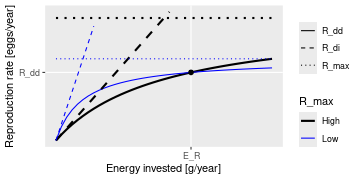
This plot shows that a given energy E_R invested into reproduction can
lead to the same reproduction rate R_{dd} with different choices
of the parameters R_max and erepro. R_max determines the asymptote of
the curve and erepro its initial slope. A higher R_max coupled with a
lower erepro (black curves) can give the same value as a lower R_max
coupled with a higher erepro (blue curves).
For the given initial state in the MizerParams object params one can
calculate the energy E_R that is invested into reproduction by the
mature individuals and the reproduction rate R_{dd} that is
required to keep the egg abundance constant. These two values determine the
location of the black dot in the above graph. You then only need one
parameter to select one curve from the family of Beverton-Holt curves going
through that point. This parameter can be erepro or R_max. Instead of
R_max you can alternatively specify the reproduction_level which is the
ratio between the density-dependent reproduction rate R_{dd} and
the maximal reproduction rate R_{max}.
If you do not provide a value for any of the reproduction parameter
arguments, then erepro will be set to the value it has in the current
species parameter data frame. If you do provide one of the reproduction
parameters, this can be either a vector with one value for each
species, or a named vector where the names determine which species are
affected, or a single unnamed value that is then used for all species. Any
species for which the given value is NA will remain unaffected.
The values for R_max must be larger than R_{dd} and can range
up to Inf. If a smaller value is requested a warning is issued and the
value is increased to the value required for a reproduction level of 0.99.
The values for the reproduction_level must be positive and
less than 1. The values for erepro must be large enough to allow the
required reproduction rate. If a smaller value is requested a warning is
issued and the value is increased to the smallest possible value. The values
for erepro should also be smaller than 1 to be physiologically sensible,
but this is not enforced by the function.
As can be seen in the graph above, choosing a lower value for R_max or a
higher value for erepro means that near the steady state the reproduction
will be less sensitive to a change in the energy invested into reproduction
and hence less sensitive to changes in the spawning stock biomass or its
energy income. As a result the species will also be less sensitive to
fishing, leading to a higher F_MSY.
Value
A MizerParams object
Examples
params <- NS_params
species_params(params)$erepro
# Attempting to set the same erepro for all species
params <- setBevertonHolt(params, erepro = 0.1)
t(species_params(params)[, c("erepro", "R_max")])
# Setting erepro for some species
params <- setBevertonHolt(params, erepro = c("Gurnard" = 0.6, "Plaice" = 0.95))
t(species_params(params)[, c("erepro", "R_max")])
# Setting R_max
R_max <- 1e17 * species_params(params)$w_max^-1
params <- setBevertonHolt(NS_params, R_max = R_max)
t(species_params(params)[, c("erepro", "R_max")])
# Setting reproduction_level
params <- setBevertonHolt(params, reproduction_level = 0.3)
t(species_params(params)[, c("erepro", "R_max")])
Set line colours and line types to be used in mizer plots
Description
Used for setting the colour and type of lines representing "Total",
"Resource", "Fishing", "Background", "External" and possibly other categories
in plots.
Usage
setColours(params, colours)

getColours(params)

setLinetypes(params, linetypes)

getLinetypes(params)
Arguments
params |
A MizerParams object |
colours |
A named list or named vector of line colours. |
linetypes |
A named list or named vector of linetypes. |
Details
Colours for names that already had a colour set for them will be overwritten by the colour you specify. Colours for names that did not yet have a colour will be appended to the list of colours.
Do not use this for setting the colours or linetypes of species, because
those are determined by setting the linecolour and linetype variables in
the species parameter data frame.
You can use the same colours in your own ggplot2 plots by adding
scale_colour_manual(values = getColours(params)) to your plot. Similarly
you can use the linetypes with
scale_linetype_manual(values = getLinetypes(params)).
Value
setColours: The MizerParams object with updated line colours
getColours(): A named vector of colours
setLinetypes(): The MizerParams object with updated linetypes
getLinetypes(): A named vector of linetypes
Examples
params <- setColours(NS_params, list("Resource" = "red","Total" = "#0000ff"))
params <- setLinetypes(NS_params, list("Total" = "dotted"))
# Set colours and linetypes for species
species_params(params)["Cod", "linecolour"] <- "black"
species_params(params)["Cod", "linetype"] <- "dashed"
plotSpectra(params, total = TRUE)
getColours(params)
getLinetypes(params)
Add a dynamical ecosystem component
Description
By default, mizer models any number of size-resolved consumer species and a single size-resolved resource spectrum. Your model may require additional components, like for example detritus or carrion or multiple resources or .... This function allows you to set up such components.
Usage
setComponent(
  params,
  component,
  initial_value,
  dynamics_fun,
  encounter_fun,
  mort_fun,
  component_params
)

removeComponent(params, component)
Arguments
params |
A MizerParams object |
component |
Name of the component |
initial_value |
Initial value of the component |
dynamics_fun |
Name of function to calculate value at the next time step |
encounter_fun |
Name of function to calculate contribution to encounter rate. Optional. |
mort_fun |
Name of function to calculate contribution to the mortality rate. Optional. |
component_params |
Object holding the parameters needed by the component functions. This could for example be a named list of parameters. Optional. |
Details
The component can be a number, a vector, an array, a list, or any other data structure you like.
If you set a component with a new name, the new component will be added
to the existing components. If you set a component with an existing name,
that component will be overwritten. You can remove a component with
removeComponent().
Value
The updated MizerParams object
Set external encounter rate
Description
Set external encounter rate
Usage
setExtEncounter(params, ext_encounter = NULL, ...)

getExtEncounter(params)

ext_encounter(params)

ext_encounter(params) <- value
Arguments
params |
MizerParams |
ext_encounter |
Optional. An array (species x size) holding the external encounter rate. If not supplied, the external encounter rate is left unchanged. Initially is is set to 0. |
... |
Unused |
value |
ext_encounter |
Value
setExtEncounter(): A MizerParams object with updated external encounter
rate.
getExtEncounter() or equivalently ext_encounter(): An array
(species x size) with the external encounter rate.
Setting external encounter rate
The external encounter rate is the rate at which a predator encounters food that is not explicitly modelled. It is a rate with units mass/year.
The ext_encounter argument allows you to specify an external encounter rate
that depends on species and body size. You can see an example of this in
the Examples section of the help page for setExtEncounter().
See Also
Other functions for setting parameters:
gear_params(),
setExtMort(),
setFishing(),
setInitialValues(),
setInteraction(),
setMaxIntakeRate(),
setMetabolicRate(),
setParams(),
setPredKernel(),
setReproduction(),
setSearchVolume(),
species_params()
Examples
params <- newMultispeciesParams(NS_species_params)

#### Setting allometric encounter rate #######################

# Set coefficient for each species. Here we choose 0.1 for each species
encounter_pre <- rep(0.1, nrow(species_params(params)))

# Multiply by power of size with exponent, here chosen to be 3/4
# The outer() function makes it an array species x size
allo_encounter <- outer(encounter_pre, w(params)^(3/4))

# Change the external encounter rate in the params object
ext_encounter(params) <- allo_encounter
Set external mortality rate
Description
Set external mortality rate
Usage
setExtMort(
  params,
  ext_mort = NULL,
  z0pre = 0.6,
  z0exp = params@resource_params$n - 1,
  reset = FALSE,
  z0 = deprecated(),
  ...
)

getExtMort(params)

ext_mort(params)

ext_mort(params) <- value
Arguments
params |
MizerParams |
ext_mort |
Optional. An array (species x size) holding the external mortality rate. If not supplied, a default is set as described in the section "Setting external mortality rate". |
z0pre |
If |
z0exp |
If |
reset |
|
z0 |
|
... |
Unused |
value |
ext_mort |
Value
setExtMort(): A MizerParams object with updated external mortality
rate.
getExtMort() or equivalently ext_mort(): An array (species x
size) with the external mortality.
Setting external mortality rate
The external mortality is all the mortality that is not due to fishing or predation by predators included in the model. The external mortality could be due to predation by predators that are not explicitly included in the model (e.g. mammals or seabirds) or due to other causes like illness. It is a rate with units 1/year.
The ext_mort argument allows you to specify an external mortality rate
that depends on species and body size. You can see an example of this in
the Examples section of the help page for setExtMort().
If the ext_mort argument is not supplied, then the external mortality is
assumed to depend only on the species, not on the size of the individual:
\mu_{ext.i}(w) = z_{0.i}. The value of the constant z_0 for each
species is taken from the z0 column of the species parameter data frame, if
that column exists. Otherwise it is calculated as
z_{0.i} = {\tt z0pre}_i\, w_{inf}^{\tt z0exp}.
See Also
Other functions for setting parameters:
gear_params(),
setExtEncounter(),
setFishing(),
setInitialValues(),
setInteraction(),
setMaxIntakeRate(),
setMetabolicRate(),
setParams(),
setPredKernel(),
setReproduction(),
setSearchVolume(),
species_params()
Examples
params <- newMultispeciesParams(NS_species_params)

#### Setting allometric death rate #######################

# Set coefficient for each species. Here we choose 0.1 for each species
z0pre <- rep(0.1, nrow(species_params(params)))

# Multiply by power of size with exponent, here chosen to be -1/4
# The outer() function makes it an array species x size
allo_mort <- outer(z0pre, w(params)^(-1/4))

# Change the external mortality rate in the params object
ext_mort(params) <- allo_mort
Set fishing parameters
Description
Set fishing parameters
Usage
setFishing(
  params,
  selectivity = NULL,
  catchability = NULL,
  reset = FALSE,
  initial_effort = NULL,
  ...
)

getCatchability(params)

catchability(params)

catchability(params) <- value

getSelectivity(params)

selectivity(params)

selectivity(params) <- value

getInitialEffort(params)
Arguments
params |
A MizerParams object |
selectivity |
Optional. An array (gear x species x size) that holds the
selectivity of each gear for species and size, |
catchability |
Optional. An array (gear x species) that holds the catchability of
each species by each gear, |
reset |
|
initial_effort |
Optional. A number or a named numeric vector specifying the fishing effort. If a number, the same effort is used for all gears. If a vector, must be named by gear. |
... |
Unused |
value |
. |
Value
setFishing(): A MizerParams object with updated fishing
parameters.
getCatchability() or equivalently catchability(): An array (gear
x species) that holds the catchability of each species by each gear,
Q_{g,i}. The names of the dimensions are "gear, "sp".
getSelectivity() or equivalently selectivity(): An array (gear x
species x size) that holds the selectivity of each gear for species and
size, S_{g,i,w}. The names of the dimensions are "gear, "sp", "w".
getInitialEffort() or equivalently initial_effort(): A named
vector with the initial fishing effort for each gear.
Setting fishing
Gears
In mizer, fishing mortality is imposed on species by fishing gears. The
total per-capita fishing mortality (1/year) is obtained by summing over the
mortality from all gears,
\mu_{f.i}(w) = \sum_g F_{g,i}(w),
where the fishing mortality F_{g,i}(w) imposed by gear g on
species i at size w is calculated as:
F_{g,i}(w) = S_{g,i}(w) Q_{g,i} E_{g},
where S is the selectivity by species, gear and size, Q is the
catchability by species and gear and E is the fishing effort by gear.
Selectivity
The selectivity at size of each gear for each species is saved as a three
dimensional array (gear x species x size). Each entry has a range between 0
(that gear is not selecting that species at that size) to 1 (that gear is
selecting all individuals of that species of that size). This three
dimensional array can be specified explicitly via the selectivity
argument, but usually mizer calculates it from the gear_params slot of
the MizerParams object.
To allow the calculation of the selectivity array, the gear_params slot
must be a data frame with one row for each gear-species combination. So if
for example a gear can select three species, then that gear contributes three
rows to the gear_params data frame, one for each species it can select. The
data frame must have columns gear, holding the name of the gear, species,
holding the name of the species, and sel_func, holding the name of the
function that calculates the selectivity curve. Some selectivity functions
are included in the package: knife_edge(), sigmoid_length(),
double_sigmoid_length(), and sigmoid_weight().
Users are able to write their own size-based selectivity function. The first
argument to the function must be w and the function must return a vector of
the selectivity (between 0 and 1) at size.
Each selectivity function may have parameters. Values for these
parameters must be included as columns in the gear parameters data.frame.
The names of the columns must exactly match the names of the corresponding
arguments of the selectivity function. For example, the default selectivity
function is knife_edge() that a has sudden change of selectivity from 0 to 1
at a certain size. In its help page you can see that the knife_edge()
function has arguments w and knife_edge_size. The first argument, w, is
size (the function calculates selectivity at size). All selectivity functions
must have w as the first argument. The values for the other arguments must
be found in the gear parameters data.frame. So for the knife_edge()
function there should be a knife_edge_size column. Because knife_edge()
is the default selectivity function, the knife_edge_size argument has a
default value = w_mat.
The most commonly-used selectivity function is sigmoid_length(). It has a
smooth transition from 0 to 1 at a certain size. The sigmoid_length()
function has the two parameters l50 and l25 that are the lengths in cm at
which 50% or 25% of the fish are selected by the gear. If you choose this
selectivity function then the l50 and l25 columns must be included in the
gear parameters data.frame.
In case each species is only selected by one gear, the columns of the
gear_params data frame can alternatively be provided as columns of the
species_params data frame, if this is more convenient for the user to set
up. Mizer will then copy these columns over to create the gear_params data
frame when it creates the MizerParams object. However changing these columns
in the species parameter data frame later will not update the gear_params
data frame.
Catchability
Catchability is used as an additional factor to make the link between gear selectivity, fishing effort and fishing mortality. For example, it can be set so that an effort of 1 gives a desired fishing mortality. In this way effort can then be specified relative to a 'base effort', e.g. the effort in a particular year.
Catchability is stored as a two dimensional array (gear x species). This can
either be provided explicitly via the catchability argument, or the
information can be provided via a catchability column in the gear_params
data frame.
In the case where each species is selected by only a single gear, the
catchability column can also be provided in the species_params data
frame. Mizer will then copy this over to the gear_params data frame when
the MizerParams object is created.
Effort
The initial fishing effort is stored in the MizerParams object. If it is
not supplied, it is set to zero. The initial effort can be overruled when
the simulation is run with project(), where it is also possible to specify
an effort that varies through time.
See Also
Other functions for setting parameters:
gear_params(),
setExtEncounter(),
setExtMort(),
setInitialValues(),
setInteraction(),
setMaxIntakeRate(),
setMetabolicRate(),
setParams(),
setPredKernel(),
setReproduction(),
setSearchVolume(),
species_params()
Examples
str(getCatchability(NS_params))
str(getSelectivity(NS_params))
str(getInitialEffort(NS_params))
Set initial values to values from a simulation
Description
This is used to use the results from one simulation as the starting values for another simulation.
Usage
setInitialValues(params, sim, time_range, geometric_mean = FALSE)
Arguments
params |
A |
sim |
A |
time_range |
The time range to average the abundances over. Can be a vector of values, a vector of min and max time, or a single value. Only the range of times is relevant, i.e., all times between the smallest and largest will be selected. Default is the final time step. |
geometric_mean |
|
Details
The initial abundances (for both species and resource) in the params
object are set to the abundances in a MizerSim object, averaged over
a range of times. Similarly, the initial effort in the params object is
set to the effort in the MizerSim object, again averaged over that range
of times.
When no time range is specified, the initial values are taken from the final
time step of the simulation.
If the model described by sim and params has additional components
created with setComponent() then the values of these components are also
averaged and copied to params.
The MizerSim object must come from a model with the same set of species and gears and other components and the same size bins as the MizerParams object. Otherwise an error is raised.
Value
The params object with updated initial values and initial effort.
Because of the way the
R language works, setInitialValues() does not make the changes to the
params object that you pass to it but instead returns a new params object.
So to affect the change you call the function in the form
params <- setInitialValues(params, sim).
See Also
Other functions for setting parameters:
gear_params(),
setExtEncounter(),
setExtMort(),
setFishing(),
setInteraction(),
setMaxIntakeRate(),
setMetabolicRate(),
setParams(),
setPredKernel(),
setReproduction(),
setSearchVolume(),
species_params()
Examples
params <- NS_params
sim <- project(params, t_max = 20, effort = 0.5)
params <- setInitialValues(params, sim)
Set species interaction matrix
Description
Set species interaction matrix
Usage
setInteraction(params, interaction = NULL)

interaction_matrix(params)

interaction_matrix(params) <- value
Arguments
params |
MizerParams object |
interaction |
Optional interaction matrix of the species (predator species x prey species). By default all entries are 1. See "Setting interaction matrix" section below. |
value |
An interaction matrix |
Value
setInteraction: A MizerParams object with updated interaction
matrix
interaction_matrix(): The interaction matrix (predator species x
prey species)
Setting interaction matrix
You do not need to specify an interaction matrix. If you do not, then the predator-prey interactions are purely determined by the size of predator and prey and totally independent of the species of predator and prey.
The interaction matrix \theta_{ij} modifies the interaction of each
pair of species in the model. This can be used for example to allow for
different spatial overlap among the species.
The values in the interaction matrix are used to scale the encountered food
and predation mortality (see on the website the section on predator-prey encounter rate
and on predation mortality).
The first index refers to the predator species and the second to the prey
species.
The interaction matrix is used when calculating the food encounter rate in
getEncounter() and the predation mortality rate in getPredMort(). Its
entries are dimensionless numbers. If all the values in the interaction
matrix are equal then predator-prey interactions are determined entirely by
size-preference.
This function checks that the supplied interaction matrix is valid and then
stores it in the interaction slot of the params object.
The order of the columns and rows of the interaction argument should be
the same as the order in the species params data frame in the params
object. If you supply a named array then the function will check the order
and warn if it is different. One way of creating your own interaction
matrix is to enter the data using a spreadsheet program and saving it as a
.csv file. The data can then be read into R using the command read.csv().
The interaction of the species with the resource are set via a column
interaction_resource in the species_params data frame. By default this
column is set to all 1s.
See Also
Other functions for setting parameters:
gear_params(),
setExtEncounter(),
setExtMort(),
setFishing(),
setInitialValues(),
setMaxIntakeRate(),
setMetabolicRate(),
setParams(),
setPredKernel(),
setReproduction(),
setSearchVolume(),
species_params()
Examples
params <- newTraitParams(no_sp = 3)
inter <- getInteraction(params)
inter[1, 2:3] <- 0
params <- setInteraction(params, interaction = inter)
getInteraction(params)
Set maximum intake rate
Description
Set maximum intake rate
Usage
setMaxIntakeRate(params, intake_max = NULL, reset = FALSE, ...)

getMaxIntakeRate(params)

intake_max(params)

intake_max(params) <- value
Arguments
params |
MizerParams |
intake_max |
Optional. An array (species x size) holding the maximum intake rate for each species at size. If not supplied, a default is set as described in the section "Setting maximum intake rate". |
reset |
|
... |
Unused |
value |
intake_max |
Value
setReproduction(): A MizerParams object with updated maximum
intake rate.
getMaxIntakeRate() or equivalently intake_max(): An array
(species x size) with the maximum intake rate.
Setting maximum intake rate
The maximum intake rate h_i(w) of an individual of species i and
weight w determines the feeding level, calculated with
getFeedingLevel(). It is measured in grams/year.
If the intake_max argument is not supplied, then the maximum intake
rate is set to
h_i(w) = h_i w^{n_i}.
The values of h_i (the maximum intake rate of an individual of size 1
gram) and n_i (the allometric exponent for the intake rate) are taken
from the h and n columns in the species parameter dataframe. If
the h column is not supplied in the species parameter dataframe, it is
calculated by the get_h_default() function.
If h_i is set to Inf, fish of species i will consume all encountered
food.
See Also
Other functions for setting parameters:
gear_params(),
setExtEncounter(),
setExtMort(),
setFishing(),
setInitialValues(),
setInteraction(),
setMetabolicRate(),
setParams(),
setPredKernel(),
setReproduction(),
setSearchVolume(),
species_params()
Set metabolic rate
Description
Sets the rate at which energy is used for metabolism and activity
Usage
setMetabolicRate(params, metab = NULL, p = NULL, reset = FALSE, ...)

getMetabolicRate(params)

metab(params)

metab(params) <- value
Arguments
params |
MizerParams |
metab |
Optional. An array (species x size) holding the metabolic rate for each species at size. If not supplied, a default is set as described in the section "Setting metabolic rate". |
p |
The allometric metabolic exponent. This is only used if |
reset |
|
... |
Unused |
value |
metab |
Value
setMetabolicRate(): A MizerParams object with updated metabolic rate.
getMetabolicRate() or equivalently metab(): An array
(species x size) with the metabolic rate.
Setting metabolic rate
The metabolic rate is subtracted from the energy income rate to calculate
the rate at which energy is available for growth and reproduction, see
getEReproAndGrowth(). It is measured in grams/year.
If the metab argument is not supplied, then for each species the
metabolic rate k(w) for an individual of size w is set to
k(w) = k_s w^p + k w,
where k_s w^p represents the rate of standard metabolism and k w
is the rate at which energy is expended on activity and movement. The values
of k_s, p and k are taken from the ks, p and
k columns in the species parameter dataframe. If any of these
parameters are not supplied, the defaults are k = 0, p = n and
k_s = f_c h \alpha w_{mat}^{n-p},
where f_c is the critical feeding level taken from the fc column
in the species parameter data frame. If the critical feeding level is not
specified, a default of f_c = 0.2 is used.
See Also
Other functions for setting parameters:
gear_params(),
setExtEncounter(),
setExtMort(),
setFishing(),
setInitialValues(),
setInteraction(),
setMaxIntakeRate(),
setParams(),
setPredKernel(),
setReproduction(),
setSearchVolume(),
species_params()
Set metadata for a model
Description
Setting metadata is particularly important for sharing your model with
others. All metadata fields are optional and you can also add other fields
of your own choosing. If you set a value
for a field that already existed, the old value will be overwritten.
Usage
setMetadata(params, title, description, authors, url, doi, ...)

getMetadata(params)
Arguments
params |
The MizerParams object for the model |
title |
A string with the title for the model |
description |
A string with a description of the model. This could for example contain information about any publications using the model. |
authors |
An author entry or a list of author entries, where each author
entry could either be just a name or could itself be a list with fields
like |
url |
A URL where more information about the model can be found. This could be a blog post on the mizer blog, for example. |
doi |
The digital object identifier for your model. To create a doi you can use online services like https://zenodo.org/ or https://figshare.com. |
... |
Additional metadata fields that you would like to add |
Details
In addition to the metadata fields you can set by hand, there are four fields that are set automatically by mizer:
-
mizer_versionThe version string of the mizer version under which the model was created or last upgraded. Can be compared to the current version which is obtained withpackageVersion("mizer"). The purpose of this field is that if the model is not working as expected in the current version of mizer, you can go back to the older version under which presumably it was working. -
extensionsA named vector of strings where each name is the name of and extension package needed to run the model and each value is a string giving the information that the remotes package needs to install the correct version of the extension package, see https://remotes.r-lib.org/. This field is set by the extension packages. -
time_createdA POSIXct date-time object with the creation time. -
time_modifiedA POSIXct date-time object with the last modified time.
Setting the metadata with this function does not count as a modification of
the object, so the time_modified field will not be updated.
Value
setMetadata(): The MizerParams object with updated metadata
getMetadata(): A list with all metadata entries that have been set,
including at least
mizer_version, extensions, time_created and time_modified.
Set or change any model parameters
Description
This is a convenient wrapper function calling each of the following functions
See the Details section below for a discussion of how to use this function.
Usage
setParams(params, interaction = NULL, ...)
Arguments
params |
A MizerParams object |
interaction |
Optional interaction matrix of the species (predator species x prey species). By default all entries are 1. See "Setting interaction matrix" section below. |
... |
Arguments passed on to
|
Details
If you are not happy with the assumptions that mizer makes by default about
the shape of the model functions, for example if you want to change one of
the allometric scaling assumptions, you can do this by providing your
choice as an array in the appropriate argument to setParams(). The
sections below discuss all the model functions that you can change this way.
Because of the way the R language works, setParams does not make the
changes to the params object that you pass to it but instead returns a new
params object. So to affect the change you call the function in the form
params <- setParams(params, ...).
Usually, if you are happy with the way mizer calculates its model functions
from the species parameters and only want to change the values of some
species parameters, you would make those changes in the species_params data
frame contained in the params object using species_params<-().
Here is an example which assumes that
you have have a MizerParams object params in which you just want to change
the gamma parameter of the third species:
species_params(params)$gamma[[3]] <- 1000
Internally that will actually call setParams() to recalculate any of the
other parameters that are affected by the change in the species parameter.
setParams() will use the species parameters in the params object to
recalculate the values of all the model functions except those for which you
have set custom values.
Value
A MizerParams object
Units in mizer
Mizer uses grams to measure weight, centimetres to measure lengths, and years to measure time.
Mizer is agnostic about whether abundances are given as
numbers per area,
numbers per volume or
total numbers for the entire study area.
You should make the choice most convenient for your application and then stick with it. If you make choice 1 or 2 you will also have to choose a unit for area or volume. Your choice will then determine the units for some of the parameters. This will be mentioned when the parameters are discussed in the sections below.
Your choice will also affect the units of the quantities you may want to
calculate with the model. For example, the yield will be in grams/year/m^2 in
case 1 if you choose m^2 as your measure of area, in grams/year/m^3 in case 2
if you choose m^3 as your unit of volume, or simply grams/year in case 3. The
same comment applies for other measures, like total biomass, which will be
grams/area in case 1, grams/volume in case 2 or simply grams in case 3. When
mizer puts units on axes in plots, it will choose the units appropriate for
case 3. So for example in plotBiomass() it gives the unit as grams.
You can convert between these choices. For example, if you use case 1, you
need to multiply with the area of the ecosystem to get the total quantity.
If you work with case 2, you need to multiply by both area and the thickness
of the productive layer. In that respect, case 2 is a bit cumbersome. The
function scaleModel() is useful to change the units you are using.
Setting interaction matrix
You do not need to specify an interaction matrix. If you do not, then the predator-prey interactions are purely determined by the size of predator and prey and totally independent of the species of predator and prey.
The interaction matrix \theta_{ij} modifies the interaction of each
pair of species in the model. This can be used for example to allow for
different spatial overlap among the species.
The values in the interaction matrix are used to scale the encountered food
and predation mortality (see on the website the section on predator-prey encounter rate
and on predation mortality).
The first index refers to the predator species and the second to the prey
species.
The interaction matrix is used when calculating the food encounter rate in
getEncounter() and the predation mortality rate in getPredMort(). Its
entries are dimensionless numbers. If all the values in the interaction
matrix are equal then predator-prey interactions are determined entirely by
size-preference.
This function checks that the supplied interaction matrix is valid and then
stores it in the interaction slot of the params object.
The order of the columns and rows of the interaction argument should be
the same as the order in the species params data frame in the params
object. If you supply a named array then the function will check the order
and warn if it is different. One way of creating your own interaction
matrix is to enter the data using a spreadsheet program and saving it as a
.csv file. The data can then be read into R using the command read.csv().
The interaction of the species with the resource are set via a column
interaction_resource in the species_params data frame. By default this
column is set to all 1s.
Setting predation kernel
Kernel dependent on predator to prey size ratio
If the pred_kernel argument is not supplied, then this function sets a
predation kernel that depends only on the ratio of predator mass to prey
mass, not on the two masses independently. The shape of that kernel is then
determined by the pred_kernel_type column in species_params.
The default for pred_kernel_type is "lognormal". This will call the function
lognormal_pred_kernel() to calculate the predation kernel.
An alternative pred_kernel type is "box", implemented by the function
box_pred_kernel(), and "power_law", implemented by the function
power_law_pred_kernel(). These functions require certain species
parameters in the species_params data frame. For the lognormal kernel these
are beta and sigma, for the box kernel they are ppmr_min
and ppmr_max. They are explained in the help pages for the kernel
functions. Except for beta and sigma, no defaults are set for
these parameters. If they are missing from the species_params data frame then
mizer will issue an error message.
You can use any other string for pred_kernel_type. If for example you
choose "my" then you need to define a function my_pred_kernel that you can
model on the existing functions like lognormal_pred_kernel().
When using a kernel that depends on the predator/prey size ratio only, mizer
does not need to store the entire three dimensional array in the MizerParams
object. Such an array can be very big when there is a large number of size
bins. Instead, mizer only needs to store two two-dimensional arrays that hold
Fourier transforms of the feeding kernel function that allow the encounter
rate and the predation rate to be calculated very efficiently. However, if
you need the full three-dimensional array you can calculate it with the
getPredKernel() function.
Kernel dependent on both predator and prey size
If you want to work with a feeding kernel that depends on predator mass and prey mass independently, you can specify the full feeding kernel as a three-dimensional array (predator species x predator size x prey size).
You should use this option only if a kernel dependent only on the predator/prey mass ratio is not appropriate. Using a kernel dependent on predator/prey mass ratio only allows mizer to use fast Fourier transform methods to significantly reduce the running time of simulations.
The order of the predator species in pred_kernel should be the same
as the order in the species params dataframe in the params object. If you
supply a named array then the function will check the order and warn if it is
different.
Setting search volume
The search volume \gamma_i(w) of an individual of species i
and weight w multiplies the predation kernel when
calculating the encounter rate in getEncounter() and the
predation rate in getPredRate().
The name "search volume" is a bit misleading, because \gamma_i(w) does
not have units of volume. It is simply a parameter that determines the rate
of predation. Its units depend on your choice, see section "Units in mizer".
If you have chosen to work with total abundances, then it is a rate with units
1/year. If you have chosen to work with abundances per m^2 then it has units
of m^2/year. If you have chosen to work with abundances per m^3 then it has
units of m^3/year.
If the search_vol argument is not supplied, then the search volume is
set to
\gamma_i(w) = \gamma_i w^q_i.
The values of \gamma_i (the search volume at 1g) and q_i (the
allometric exponent of the search volume) are taken from the gamma and
q columns in the species parameter dataframe. If the gamma
column is not supplied in the species parameter dataframe, a default is
calculated by the get_gamma_default() function. Note that only
for predators of size w = 1 gram is the value of the species parameter
\gamma_i the same as the value of the search volume \gamma_i(w).
Setting maximum intake rate
The maximum intake rate h_i(w) of an individual of species i and
weight w determines the feeding level, calculated with
getFeedingLevel(). It is measured in grams/year.
If the intake_max argument is not supplied, then the maximum intake
rate is set to
h_i(w) = h_i w^{n_i}.
The values of h_i (the maximum intake rate of an individual of size 1
gram) and n_i (the allometric exponent for the intake rate) are taken
from the h and n columns in the species parameter dataframe. If
the h column is not supplied in the species parameter dataframe, it is
calculated by the get_h_default() function.
If h_i is set to Inf, fish of species i will consume all encountered
food.
Setting metabolic rate
The metabolic rate is subtracted from the energy income rate to calculate
the rate at which energy is available for growth and reproduction, see
getEReproAndGrowth(). It is measured in grams/year.
If the metab argument is not supplied, then for each species the
metabolic rate k(w) for an individual of size w is set to
k(w) = k_s w^p + k w,
where k_s w^p represents the rate of standard metabolism and k w
is the rate at which energy is expended on activity and movement. The values
of k_s, p and k are taken from the ks, p and
k columns in the species parameter dataframe. If any of these
parameters are not supplied, the defaults are k = 0, p = n and
k_s = f_c h \alpha w_{mat}^{n-p},
where f_c is the critical feeding level taken from the fc column
in the species parameter data frame. If the critical feeding level is not
specified, a default of f_c = 0.2 is used.
Setting external mortality rate
The external mortality is all the mortality that is not due to fishing or predation by predators included in the model. The external mortality could be due to predation by predators that are not explicitly included in the model (e.g. mammals or seabirds) or due to other causes like illness. It is a rate with units 1/year.
The ext_mort argument allows you to specify an external mortality rate
that depends on species and body size. You can see an example of this in
the Examples section of the help page for setExtMort().
If the ext_mort argument is not supplied, then the external mortality is
assumed to depend only on the species, not on the size of the individual:
\mu_{ext.i}(w) = z_{0.i}. The value of the constant z_0 for each
species is taken from the z0 column of the species parameter data frame, if
that column exists. Otherwise it is calculated as
z_{0.i} = {\tt z0pre}_i\, w_{inf}^{\tt z0exp}.
Setting external encounter rate
The external encounter rate is the rate at which a predator encounters food that is not explicitly modelled. It is a rate with units mass/year.
The ext_encounter argument allows you to specify an external encounter rate
that depends on species and body size. You can see an example of this in
the Examples section of the help page for setExtEncounter().
Setting reproduction
For each species and at each size, the proportion \psi of the
available energy
that is invested into reproduction is the product of two factors: the
proportion maturity of individuals that are mature and the proportion
repro_prop of the energy available to a mature individual that is
invested into reproduction. There is a size w_repro_max at which all the
energy is invested into reproduction and therefore all growth stops. There
can be no fish larger than w_repro_max. If you have not specified the
w_repro_max column in the species parameter data frame, then the maximum size
w_max is used instead.
Maturity ogive
If the the proportion of individuals that are mature is not supplied via
the maturity argument, then it is set to a sigmoidal
maturity ogive that changes from 0 to 1 at around the maturity size:
{\tt maturity}(w) = \left[1+\left(\frac{w}{w_{mat}}\right)^{-U}\right]^{-1}.
(To avoid clutter, we are not showing the species index in the equations,
although each species has its own maturity ogive.)
The maturity weights are taken from the w_mat column of the
species_params data frame. Any missing maturity weights are set to 1/4 of the
maximum weight in the w_max column.
The exponent U determines the steepness of the maturity ogive. By
default it is chosen as U = 10, however this can be overridden by
including a column w_mat25 in the species parameter dataframe that
specifies the weight at which 25% of individuals are mature, which sets
U = \log(3) / \log(w_{mat} / w_{mat25}).
The sigmoidal function given above would strictly reach 1 only
asymptotically. Mizer instead sets the function equal to 1 already at a size
taken from the w_repro_max column in the species parameter data frame, if it
exists, or otherwise from the w_max column. Also, for computational
simplicity, any proportion smaller than 1e-8 is set to 0.
Investment into reproduction
If the the energy available to a mature individual that is
invested into reproduction is not supplied via the repro_prop argument,
it is set to the allometric form
{\tt repro\_prop}(w) = \left(\frac{w}{w_{\tt{repro\_max}}}\right)^{m-n}.
Here n is the scaling exponent of the energy income rate. Hence
the exponent m determines the scaling of the investment into
reproduction for mature individuals. By default it is chosen to be
m = 1 so that the rate at which energy is invested into reproduction
scales linearly with the size. This default can be overridden by including a
column m in the species parameter dataframe. The maximum sizes are taken
from the w_repro_max column in the species parameter data frame, if it
exists, or otherwise from the w_max column.
The total proportion of energy invested into reproduction of an individual
of size w is then
\psi(w) = {\tt maturity}(w){\tt repro\_prop}(w)
Reproductive efficiency
The reproductive efficiency \epsilon, i.e., the proportion of energy allocated to
reproduction that results in egg biomass, is set through the erepro
column in the species_params data frame. If that is not provided, the default
is set to 1 (which you will want to override). The offspring biomass divided
by the egg biomass gives the rate of egg production, returned by
getRDI():
R_{di} = \frac{\epsilon}{2 w_{min}} \int N(w) E_r(w) \psi(w) \, dw
Density dependence
The stock-recruitment relationship is an emergent phenomenon in mizer, with several sources of density dependence. Firstly, the amount of energy invested into reproduction depends on the energy income of the spawners, which is density-dependent due to competition for prey. Secondly, the proportion of larvae that grow up to recruitment size depends on the larval mortality, which depends on the density of predators, and on larval growth rate, which depends on density of prey.
Finally, to encode all the density dependence in the stock-recruitment
relationship that is not already included in the other two sources of density
dependence, mizer puts the the density-independent rate of egg production
through a density-dependence function. The result is returned by
getRDD(). The name of the density-dependence function is
specified by the RDD argument. The default is the Beverton-Holt
function BevertonHoltRDD(), which requires an R_max column
in the species_params data frame giving the maximum egg production rate. If
this column does not exist, it is initialised to Inf, leading to no
density-dependence. Other functions provided by mizer are
RickerRDD() and SheperdRDD() and you can easily use
these as models for writing your own functions.
Setting fishing
Gears
In mizer, fishing mortality is imposed on species by fishing gears. The
total per-capita fishing mortality (1/year) is obtained by summing over the
mortality from all gears,
\mu_{f.i}(w) = \sum_g F_{g,i}(w),
where the fishing mortality F_{g,i}(w) imposed by gear g on
species i at size w is calculated as:
F_{g,i}(w) = S_{g,i}(w) Q_{g,i} E_{g},
where S is the selectivity by species, gear and size, Q is the
catchability by species and gear and E is the fishing effort by gear.
Selectivity
The selectivity at size of each gear for each species is saved as a three
dimensional array (gear x species x size). Each entry has a range between 0
(that gear is not selecting that species at that size) to 1 (that gear is
selecting all individuals of that species of that size). This three
dimensional array can be specified explicitly via the selectivity
argument, but usually mizer calculates it from the gear_params slot of
the MizerParams object.
To allow the calculation of the selectivity array, the gear_params slot
must be a data frame with one row for each gear-species combination. So if
for example a gear can select three species, then that gear contributes three
rows to the gear_params data frame, one for each species it can select. The
data frame must have columns gear, holding the name of the gear, species,
holding the name of the species, and sel_func, holding the name of the
function that calculates the selectivity curve. Some selectivity functions
are included in the package: knife_edge(), sigmoid_length(),
double_sigmoid_length(), and sigmoid_weight().
Users are able to write their own size-based selectivity function. The first
argument to the function must be w and the function must return a vector of
the selectivity (between 0 and 1) at size.
Each selectivity function may have parameters. Values for these
parameters must be included as columns in the gear parameters data.frame.
The names of the columns must exactly match the names of the corresponding
arguments of the selectivity function. For example, the default selectivity
function is knife_edge() that a has sudden change of selectivity from 0 to 1
at a certain size. In its help page you can see that the knife_edge()
function has arguments w and knife_edge_size. The first argument, w, is
size (the function calculates selectivity at size). All selectivity functions
must have w as the first argument. The values for the other arguments must
be found in the gear parameters data.frame. So for the knife_edge()
function there should be a knife_edge_size column. Because knife_edge()
is the default selectivity function, the knife_edge_size argument has a
default value = w_mat.
The most commonly-used selectivity function is sigmoid_length(). It has a
smooth transition from 0 to 1 at a certain size. The sigmoid_length()
function has the two parameters l50 and l25 that are the lengths in cm at
which 50% or 25% of the fish are selected by the gear. If you choose this
selectivity function then the l50 and l25 columns must be included in the
gear parameters data.frame.
In case each species is only selected by one gear, the columns of the
gear_params data frame can alternatively be provided as columns of the
species_params data frame, if this is more convenient for the user to set
up. Mizer will then copy these columns over to create the gear_params data
frame when it creates the MizerParams object. However changing these columns
in the species parameter data frame later will not update the gear_params
data frame.
Catchability
Catchability is used as an additional factor to make the link between gear selectivity, fishing effort and fishing mortality. For example, it can be set so that an effort of 1 gives a desired fishing mortality. In this way effort can then be specified relative to a 'base effort', e.g. the effort in a particular year.
Catchability is stored as a two dimensional array (gear x species). This can
either be provided explicitly via the catchability argument, or the
information can be provided via a catchability column in the gear_params
data frame.
In the case where each species is selected by only a single gear, the
catchability column can also be provided in the species_params data
frame. Mizer will then copy this over to the gear_params data frame when
the MizerParams object is created.
Effort
The initial fishing effort is stored in the MizerParams object. If it is
not supplied, it is set to zero. The initial effort can be overruled when
the simulation is run with project(), where it is also possible to specify
an effort that varies through time.
See Also
Other functions for setting parameters:
gear_params(),
setExtEncounter(),
setExtMort(),
setFishing(),
setInitialValues(),
setInteraction(),
setMaxIntakeRate(),
setMetabolicRate(),
setPredKernel(),
setReproduction(),
setSearchVolume(),
species_params()
Set predation kernel
Description
The predation kernel determines the distribution of prey sizes that a
predator feeds on. It is used in getEncounter() when calculating
the rate at which food is encountered and in getPredRate() when
calculating the rate at which a prey is predated upon. The predation kernel
can be a function of the predator/prey size ratio or it can be a function of
the predator size and the prey size separately. Both types can be set up with
this function.
Usage
setPredKernel(params, pred_kernel = NULL, reset = FALSE, ...)

getPredKernel(params)

pred_kernel(params)

pred_kernel(params) <- value
Arguments
params |
A MizerParams object |
pred_kernel |
Optional. An array (species x predator size x prey size) that holds the predation coefficient of each predator at size on each prey size. If not supplied, a default is set as described in section "Setting predation kernel". |
reset |
|
... |
Unused |
value |
pred_kernel |
Value
setPredKernel(): A MizerParams object with updated predation kernel.
getPredKernel() or equivalently pred_kernel(): An array (predator
species x predator_size x prey_size)
Setting predation kernel
Kernel dependent on predator to prey size ratio
If the pred_kernel argument is not supplied, then this function sets a
predation kernel that depends only on the ratio of predator mass to prey
mass, not on the two masses independently. The shape of that kernel is then
determined by the pred_kernel_type column in species_params.
The default for pred_kernel_type is "lognormal". This will call the function
lognormal_pred_kernel() to calculate the predation kernel.
An alternative pred_kernel type is "box", implemented by the function
box_pred_kernel(), and "power_law", implemented by the function
power_law_pred_kernel(). These functions require certain species
parameters in the species_params data frame. For the lognormal kernel these
are beta and sigma, for the box kernel they are ppmr_min
and ppmr_max. They are explained in the help pages for the kernel
functions. Except for beta and sigma, no defaults are set for
these parameters. If they are missing from the species_params data frame then
mizer will issue an error message.
You can use any other string for pred_kernel_type. If for example you
choose "my" then you need to define a function my_pred_kernel that you can
model on the existing functions like lognormal_pred_kernel().
When using a kernel that depends on the predator/prey size ratio only, mizer
does not need to store the entire three dimensional array in the MizerParams
object. Such an array can be very big when there is a large number of size
bins. Instead, mizer only needs to store two two-dimensional arrays that hold
Fourier transforms of the feeding kernel function that allow the encounter
rate and the predation rate to be calculated very efficiently. However, if
you need the full three-dimensional array you can calculate it with the
getPredKernel() function.
Kernel dependent on both predator and prey size
If you want to work with a feeding kernel that depends on predator mass and prey mass independently, you can specify the full feeding kernel as a three-dimensional array (predator species x predator size x prey size).
You should use this option only if a kernel dependent only on the predator/prey mass ratio is not appropriate. Using a kernel dependent on predator/prey mass ratio only allows mizer to use fast Fourier transform methods to significantly reduce the running time of simulations.
The order of the predator species in pred_kernel should be the same
as the order in the species params dataframe in the params object. If you
supply a named array then the function will check the order and warn if it is
different.
See Also
Other functions for setting parameters:
gear_params(),
setExtEncounter(),
setExtMort(),
setFishing(),
setInitialValues(),
setInteraction(),
setMaxIntakeRate(),
setMetabolicRate(),
setParams(),
setReproduction(),
setSearchVolume(),
species_params()
Examples
## Set up a MizerParams object
params <-  NS_params

## If you change predation kernel parameters after setting up a model,
#  this will be used to recalculate the kernel
species_params(params)["Cod", "beta"] <- 200

## You can change to a different predation kernel type
species_params(params)$ppmr_max <- 4000
species_params(params)$ppmr_min <- 200
species_params(params)$pred_kernel_type <- "box"
plot(w_full(params), getPredKernel(params)["Cod", 100, ], type="l", log="x")

## If you need a kernel that depends also on prey size you need to define
# it yourself.
pred_kernel <- getPredKernel(params)
pred_kernel["Herring", , ] <- sweep(pred_kernel["Herring", , ], 2,
                                    params@w_full, "*")
params<- setPredKernel(params, pred_kernel = pred_kernel)
Set own rate function to replace mizer rate function
Description
If the way mizer calculates a fundamental rate entering the model is
not flexible enough for you (for example if you need to introduce time
dependence) then you can write your own functions for calculating that
rate and use setRateFunction() to register it with mizer.
Usage
setRateFunction(params, rate, fun)

getRateFunction(params, rate)

other_params(params)

other_params(params) <- value
Arguments
params |
A MizerParams object |
rate |
Name of the rate for which a new function is to be set. |
fun |
Name of the function to use to calculate the rate. |
value |
Values for other parameters |
Details
At each time step during a simulation with the project() function, mizer
needs to calculate the instantaneous values of the various rates. By
default it calls the mizerRates() function which creates a list with the
following components:
-
encounterfrommizerEncounter() -
feeding_levelfrommizerFeedingLevel() -
pred_ratefrommizerPredRate() -
pred_mortfrommizerPredMort() -
f_mortfrommizerFMort() -
mortfrommizerMort() -
resource_mortfrommizerResourceMort() -
efrommizerEReproAndGrowth() -
e_reprofrommizerERepro() -
e_growthfrommizerEGrowth() -
rdifrommizerRDI() -
rddfromBevertonHoltRDD()
For each of these you can substitute your own function. So for example if
you have written your own function for calculating the total mortality
rate and have called it myMort and have a mizer model stored in a
MizerParams object called params that you want to run with your new
mortality rate, then you would call
params <- setRateFunction(params, "Mort", "myMort")
In general if you want to replace a function mizerSomeRateFunc() with
a function myVersionOfThis() you would call
params <- setRateFunction(params, "SomeRateFunc", "myVersionOfThis")
In some extreme cases you may need to swap out the entire mizerRates()
function for your own function called myRates(). That you can do with
params <- setRateFunction(params, "Rates", "myRates")
Your new rate functions may need their own model parameters. These you
can store in other_params(params). For example
other_params(params)$my_param <- 42
Note that your own rate functions need to be defined in the global environment or in a package. If they are defined within a function then mizer will not find them.
Value
For setRateFunction(): An updated MizerParams object
For getRateFunction(): The name of the registered rate function for
the requested rate, or the list of all rate functions if called without
rate argument.
For other_params(): A named list with all the parameters for which
you have set values.
Set reproduction parameters
Description
Sets the proportion of the total energy available for reproduction and growth that is invested into reproduction as a function of the size of the individual and sets additional density dependence.
Usage
setReproduction(
  params,
  maturity = NULL,
  repro_prop = NULL,
  reset = FALSE,
  RDD = NULL,
  ...
)

getMaturityProportion(params)

maturity(params)

maturity(params) <- value

getReproductionProportion(params)

repro_prop(params)

repro_prop(params) <- value
Arguments
params |
A MizerParams object |
maturity |
Optional. An array (species x size) that holds the proportion of individuals of each species at size that are mature. If not supplied, a default is set as described in the section "Setting reproduction". |
repro_prop |
Optional. An array (species x size) that holds the proportion of consumed energy that a mature individual allocates to reproduction for each species at size. If not supplied, a default is set as described in the section "Setting reproduction". |
reset |
|
RDD |
The name of the function calculating the density-dependent
reproduction rate from the density-independent rate. Defaults to
" |
... |
Unused |
value |
. |
Value
setReproduction(): A MizerParams object with updated reproduction
parameters.
getMaturityProportion() or equivalently 'maturity():
An array (species x size) that holds the proportion
of individuals of each species at size that are mature.
getReproductionProportion() or equivalently repro_prop():
An array (species x size) that holds the
proportion of consumed energy that a mature individual allocates to
reproduction for each species at size. For sizes where the maturity
proportion is zero, also the reproduction proportion is returned as zero.
Setting reproduction
For each species and at each size, the proportion \psi of the
available energy
that is invested into reproduction is the product of two factors: the
proportion maturity of individuals that are mature and the proportion
repro_prop of the energy available to a mature individual that is
invested into reproduction. There is a size w_repro_max at which all the
energy is invested into reproduction and therefore all growth stops. There
can be no fish larger than w_repro_max. If you have not specified the
w_repro_max column in the species parameter data frame, then the maximum size
w_max is used instead.
Maturity ogive
If the the proportion of individuals that are mature is not supplied via
the maturity argument, then it is set to a sigmoidal
maturity ogive that changes from 0 to 1 at around the maturity size:
{\tt maturity}(w) = \left[1+\left(\frac{w}{w_{mat}}\right)^{-U}\right]^{-1}.
(To avoid clutter, we are not showing the species index in the equations,
although each species has its own maturity ogive.)
The maturity weights are taken from the w_mat column of the
species_params data frame. Any missing maturity weights are set to 1/4 of the
maximum weight in the w_max column.
The exponent U determines the steepness of the maturity ogive. By
default it is chosen as U = 10, however this can be overridden by
including a column w_mat25 in the species parameter dataframe that
specifies the weight at which 25% of individuals are mature, which sets
U = \log(3) / \log(w_{mat} / w_{mat25}).
The sigmoidal function given above would strictly reach 1 only
asymptotically. Mizer instead sets the function equal to 1 already at a size
taken from the w_repro_max column in the species parameter data frame, if it
exists, or otherwise from the w_max column. Also, for computational
simplicity, any proportion smaller than 1e-8 is set to 0.
Investment into reproduction
If the the energy available to a mature individual that is
invested into reproduction is not supplied via the repro_prop argument,
it is set to the allometric form
{\tt repro\_prop}(w) = \left(\frac{w}{w_{\tt{repro\_max}}}\right)^{m-n}.
Here n is the scaling exponent of the energy income rate. Hence
the exponent m determines the scaling of the investment into
reproduction for mature individuals. By default it is chosen to be
m = 1 so that the rate at which energy is invested into reproduction
scales linearly with the size. This default can be overridden by including a
column m in the species parameter dataframe. The maximum sizes are taken
from the w_repro_max column in the species parameter data frame, if it
exists, or otherwise from the w_max column.
The total proportion of energy invested into reproduction of an individual
of size w is then
\psi(w) = {\tt maturity}(w){\tt repro\_prop}(w)
Reproductive efficiency
The reproductive efficiency \epsilon, i.e., the proportion of energy allocated to
reproduction that results in egg biomass, is set through the erepro
column in the species_params data frame. If that is not provided, the default
is set to 1 (which you will want to override). The offspring biomass divided
by the egg biomass gives the rate of egg production, returned by
getRDI():
R_{di} = \frac{\epsilon}{2 w_{min}} \int N(w) E_r(w) \psi(w) \, dw
Density dependence
The stock-recruitment relationship is an emergent phenomenon in mizer, with several sources of density dependence. Firstly, the amount of energy invested into reproduction depends on the energy income of the spawners, which is density-dependent due to competition for prey. Secondly, the proportion of larvae that grow up to recruitment size depends on the larval mortality, which depends on the density of predators, and on larval growth rate, which depends on density of prey.
Finally, to encode all the density dependence in the stock-recruitment
relationship that is not already included in the other two sources of density
dependence, mizer puts the the density-independent rate of egg production
through a density-dependence function. The result is returned by
getRDD(). The name of the density-dependence function is
specified by the RDD argument. The default is the Beverton-Holt
function BevertonHoltRDD(), which requires an R_max column
in the species_params data frame giving the maximum egg production rate. If
this column does not exist, it is initialised to Inf, leading to no
density-dependence. Other functions provided by mizer are
RickerRDD() and SheperdRDD() and you can easily use
these as models for writing your own functions.
See Also
Other functions for setting parameters:
gear_params(),
setExtEncounter(),
setExtMort(),
setFishing(),
setInitialValues(),
setInteraction(),
setMaxIntakeRate(),
setMetabolicRate(),
setParams(),
setPredKernel(),
setSearchVolume(),
species_params()
Examples
# Plot maturity and reproduction ogives for Cod in North Sea model
maturity <- getMaturityProportion(NS_params)["Cod", ]
repro_prop <- getReproductionProportion(NS_params)["Cod", ]
df <- data.frame(Size = w(NS_params),
                 Reproduction = repro_prop,
                 Maturity = maturity,
                 Total = maturity * repro_prop)
dff <- melt(df, id.vars = "Size",
            variable.name = "Type",
            value.name = "Proportion")
library(ggplot2)
ggplot(dff) + geom_line(aes(x = Size, y = Proportion, colour = Type))
Set resource dynamics
Description
Sets the intrinsic resource birth rate and the intrinsic resource carrying
capacity as well as the name of the function used to simulate the resource
dynamics. By default, the birth rate and the carrying capacity are changed
together in such a way that the resource replenishes at the same rate at
which it is consumed. So you should only provide either the
resource_rate or the resource_capacity (or resource_level) because
the other is determined by the requirement that the resource replenishes
at the same rate at which it is consumed.
Usage
setResource(
  params,
  resource_rate = NULL,
  resource_capacity = NULL,
  resource_level = NULL,
  resource_dynamics = NULL,
  balance = NULL,
  lambda = resource_params(params)[["lambda"]],
  n = resource_params(params)[["n"]],
  w_pp_cutoff = resource_params(params)[["w_pp_cutoff"]],
  r_pp = deprecated(),
  kappa = deprecated(),
  ...
)

resource_rate(params)

resource_rate(params) <- value

resource_capacity(params)

resource_capacity(params) <- value

resource_level(params)

resource_level(params) <- value

resource_dynamics(params)

resource_dynamics(params) <- value
Arguments
params |
A MizerParams object |
resource_rate |
Optional. A vector of per-capita resource birth rate for each size class or a single number giving the coefficient in the power-law for this rate, see "Setting resource dynamics" below. Must be strictly positive. |
resource_capacity |
Optional. Vector of resource intrinsic carrying capacities or coefficient in the power-law for the capacity, see "Setting resource dynamics" below. The resource capacity must be larger than the resource abundance. |
resource_level |
Optional. The ratio between the current resource number
density and the resource capacity. Either a number used at all sizes or a
vector specifying a value for each size. Must be strictly between 0 and 1,
except at sizes where the resource is zero, where it can be |
resource_dynamics |
Optional. Name of the function that determines the resource dynamics by calculating the resource spectrum at the next time step from the current state. |
balance |
By default, if possible, the resource parameters are set so that the resource replenishes at the same rate at which it is consumed. In this case you should only specify either the resource rate or the resource capacity (or resource level) because the other is then determined automatically. Set to FALSE if you do not want the balancing. |
lambda |
Used to set power-law exponent for resource capacity if the
|
n |
Used to set power-law exponent for resource rate if the
|
w_pp_cutoff |
The upper cut off size of the resource spectrum power law
used when |
r_pp |
|
kappa |
|
... |
Unused |
value |
The desired new value for the respective parameter. |
Details
You would usually set the resource dynamics only after having finished the
calibration of the steady state. Then setting the resource dynamics with
this function will preserve that steady state, unless you explicitly
choose to set balance = FALSE. Your choice of the resource dynamics only
affects the dynamics around the steady state. The higher the resource rate
or the lower the resource capacity the less sensitive the model will be to
changes in the competition for resource.
If you provide the resource_level then that sets the resource_capacity
to the current resource number density divided by the resource level. So
in that case you should not specify resource_capacity as well.
If you provide none of the arguments resource_level, resource_rate or
resource_capacity then the resource rate is kept at its previous value.
Value
setResource: A MizerParams object with updated resource parameters
A vector with the intrinsic resource birth rate for each size class.
A vector with the intrinsic resource capacity for each size class.
A vector with the ratio between the current resource number density and the resource capacity for each size class.
The name of the function that determines the resource dynamics.
Setting resource dynamics
The resource_dynamics argument allows you to choose the resource dynamics
function. By default, mizer uses a semichemostat model to describe the
resource dynamics in each size class independently. This semichemostat
dynamics is implemented by the function resource_semichemostat(). You can
change that to use a logistic model implemented by resource_logistic() or
you can use resource_constant() which keeps the resource constant or you
can write your own function.
Both the resource_semichemostat() and the resource_logistic() dynamics
are parametrised in terms of a size-dependent birth rate r_R(w) and a
size-dependent capacity c_R. The help pages of these functions give
the details.
The resource_rate argument can be a vector (with the same length as
w_full(params)) specifying the intrinsic resource birth rate for each size
class. Alternatively it can be a single number that is used as the
coefficient in a power law: then the intrinsic birth rate r_R(w) at
size w is set to
r_R(w) = r_R w^{n-1}.
The power-law exponent n is taken from the n argument.
The resource_capacity argument can be a vector specifying the intrinsic
resource carrying capacity for each size class. Alternatively it can be a
single number that is used as the coefficient in a truncated power
law: then the intrinsic carrying capacity c_R(w) at size w
is set to
c_R(w) = c_R\, w^{-\lambda}
for all w less than w_pp_cutoff and zero for larger sizes.
The power-law exponent \lambda is taken from the lambda argument.
The values for lambda, n and w_pp_cutoff are stored in a list
in the resource_params slot of the MizerParams object so that they can be
re-used automatically in the future. That list can be accessed with
resource_params().
See Also
Examples
params <- NS_params
resource_dynamics(params)
resource_dynamics(params) <- "resource_constant"
Alias for setBevertonHolt()
Description
An alias provided for backward compatibility with mizer version <= 2.0.4
Usage
setRmax(params, R_factor = deprecated(), erepro, R_max, reproduction_level)
Arguments
params |
A MizerParams object |
R_factor |
|
erepro |
Reproductive efficiency for each species. See details. |
R_max |
Maximum reproduction rate. See details. |
reproduction_level |
Sets |
Details
With Beverton-Holt density dependence the relation between the energy
invested into reproduction and the number of eggs hatched is determined
by two parameters: the reproductive efficiency erepro and the maximum
reproduction rate R_max.
If no maximum is imposed on the reproduction rate
(R_{max} = \infty) then the resulting density-independent
reproduction rate R_{di} is proportional
to the total rate E_R at which energy is invested into reproduction,
R_{di} = \frac{\rm{erepro}}{2 w_{min}} E_R,
where the proportionality factor is given by the reproductive efficiency
erepro divided by the egg size w_min to convert energy to egg number and
divided by 2 to account for the two sexes.
Imposing a finite maximum reproduction rate R_{max} leads to a
non-linear relationship between energy invested and eggs hatched. This
density-dependent reproduction rate R_{dd} is given as
R_{dd} = R_{di}
\frac{R_{max}}{R_{di} + R_{max}}.
(All quantities in the above equations are species-specific but we dropped the species index for simplicity.)
The following plot illustrates the Beverton-Holt density dependence in the
reproduction rate for two different choices of parameters.
This plot shows that a given energy E_R invested into reproduction can
lead to the same reproduction rate R_{dd} with different choices
of the parameters R_max and erepro. R_max determines the asymptote of
the curve and erepro its initial slope. A higher R_max coupled with a
lower erepro (black curves) can give the same value as a lower R_max
coupled with a higher erepro (blue curves).
For the given initial state in the MizerParams object params one can
calculate the energy E_R that is invested into reproduction by the
mature individuals and the reproduction rate R_{dd} that is
required to keep the egg abundance constant. These two values determine the
location of the black dot in the above graph. You then only need one
parameter to select one curve from the family of Beverton-Holt curves going
through that point. This parameter can be erepro or R_max. Instead of
R_max you can alternatively specify the reproduction_level which is the
ratio between the density-dependent reproduction rate R_{dd} and
the maximal reproduction rate R_{max}.
If you do not provide a value for any of the reproduction parameter
arguments, then erepro will be set to the value it has in the current
species parameter data frame. If you do provide one of the reproduction
parameters, this can be either a vector with one value for each
species, or a named vector where the names determine which species are
affected, or a single unnamed value that is then used for all species. Any
species for which the given value is NA will remain unaffected.
The values for R_max must be larger than R_{dd} and can range
up to Inf. If a smaller value is requested a warning is issued and the
value is increased to the value required for a reproduction level of 0.99.
The values for the reproduction_level must be positive and
less than 1. The values for erepro must be large enough to allow the
required reproduction rate. If a smaller value is requested a warning is
issued and the value is increased to the smallest possible value. The values
for erepro should also be smaller than 1 to be physiologically sensible,
but this is not enforced by the function.
As can be seen in the graph above, choosing a lower value for R_max or a
higher value for erepro means that near the steady state the reproduction
will be less sensitive to a change in the energy invested into reproduction
and hence less sensitive to changes in the spawning stock biomass or its
energy income. As a result the species will also be less sensitive to
fishing, leading to a higher F_MSY.
Value
A MizerParams object
Examples
params <- NS_params
species_params(params)$erepro
# Attempting to set the same erepro for all species
params <- setBevertonHolt(params, erepro = 0.1)
t(species_params(params)[, c("erepro", "R_max")])
# Setting erepro for some species
params <- setBevertonHolt(params, erepro = c("Gurnard" = 0.6, "Plaice" = 0.95))
t(species_params(params)[, c("erepro", "R_max")])
# Setting R_max
R_max <- 1e17 * species_params(params)$w_max^-1
params <- setBevertonHolt(NS_params, R_max = R_max)
t(species_params(params)[, c("erepro", "R_max")])
# Setting reproduction_level
params <- setBevertonHolt(params, reproduction_level = 0.3)
t(species_params(params)[, c("erepro", "R_max")])
Set search volume
Description
Set search volume
Usage
setSearchVolume(params, search_vol = NULL, reset = FALSE, ...)

getSearchVolume(params)

search_vol(params)

search_vol(params) <- value
Arguments
params |
MizerParams |
search_vol |
Optional. An array (species x size) holding the search volume for each species at size. If not supplied, a default is set as described in the section "Setting search volume". |
reset |
|
... |
Unused |
value |
search_vol |
Value
setSearchVolume(): A MizerParams object with updated search volume.
getSearchVolume() or equivalently search_vol(): An array (species
x size) holding the search volume
Setting search volume
The search volume \gamma_i(w) of an individual of species i
and weight w multiplies the predation kernel when
calculating the encounter rate in getEncounter() and the
predation rate in getPredRate().
The name "search volume" is a bit misleading, because \gamma_i(w) does
not have units of volume. It is simply a parameter that determines the rate
of predation. Its units depend on your choice, see section "Units in mizer".
If you have chosen to work with total abundances, then it is a rate with units
1/year. If you have chosen to work with abundances per m^2 then it has units
of m^2/year. If you have chosen to work with abundances per m^3 then it has
units of m^3/year.
If the search_vol argument is not supplied, then the search volume is
set to
\gamma_i(w) = \gamma_i w^q_i.
The values of \gamma_i (the search volume at 1g) and q_i (the
allometric exponent of the search volume) are taken from the gamma and
q columns in the species parameter dataframe. If the gamma
column is not supplied in the species parameter dataframe, a default is
calculated by the get_gamma_default() function. Note that only
for predators of size w = 1 gram is the value of the species parameter
\gamma_i the same as the value of the search volume \gamma_i(w).
See Also
Other functions for setting parameters:
gear_params(),
setExtEncounter(),
setExtMort(),
setFishing(),
setInitialValues(),
setInteraction(),
setMaxIntakeRate(),
setMetabolicRate(),
setParams(),
setPredKernel(),
setReproduction(),
species_params()
Deprecated function for setting up parameters for a community-type model
Description
This function has been deprecated in favour of the function
newCommunityParams() that sets better default values.
Usage
set_community_model(
  max_w = 1e+06,
  min_w = 0.001,
  min_w_pp = 1e-10,
  z0 = 0.1,
  alpha = 0.2,
  h = 10,
  beta = 100,
  sigma = 2,
  q = 0.8,
  n = 2/3,
  kappa = 1000,
  lambda = 2 + q - n,
  f0 = 0.7,
  r_pp = 10,
  gamma = NA,
  knife_edge_size = 1000,
  knife_is_min = TRUE,
  recruitment = kappa * min_w^-lambda,
  rec_mult = 1,
  ...
)
Arguments
max_w |
The maximum size of the community. The |
min_w |
The minimum size of the community. Default value is 1e-3. |
min_w_pp |
The smallest size of the resource spectrum. |
z0 |
The background mortality of the community. Default value is 0.1. |
alpha |
The assimilation efficiency of the community. Default value 0.2 |
h |
The maximum food intake rate. Default value is 10. |
beta |
The preferred predator prey mass ratio. Default value is 100. |
sigma |
The width of the prey preference. Default value is 2.0. |
q |
The search volume exponent. Default value is 0.8. |
n |
The scaling of the intake. Default value is 2/3. |
kappa |
The carrying capacity of the resource spectrum. Default value is 1000. |
lambda |
The exponent of the resource spectrum. Default value is 2 + q - n. |
f0 |
The average feeding level of individuals who feed on a power-law
spectrum. This value is used to calculate the search rate parameter
|
r_pp |
Growth rate parameter for the resource spectrum. Default value is 10. |
gamma |
Volumetric search rate. Estimated using |
knife_edge_size |
The size at the edge of the knife-selectivity function. Default value is 1000. |
knife_is_min |
Is the knife-edge selectivity function selecting above (TRUE) or below (FALSE) the edge. Default is TRUE. |
recruitment |
The constant recruitment in the smallest size class of the
community spectrum. This should be set so that the community spectrum
continues the resource spectrum. Default value = |
rec_mult |
Additional multiplier for the constant recruitment. Default value is 1. |
... |
Other arguments to pass to the |
Details
This functions creates a MizerParams object so that
community-type models can be easily set up and run. A community model has
several features that distinguish it from the food-web type models. Only one
'species' is resolved, i.e. one 'species' is used to represent the whole
community. The resource spectrum only extends to the start of the community
spectrum. Recruitment to the smallest size in the community spectrum is
constant and set by the user. As recruitment is constant, the proportion of
energy invested in reproduction (the slot psi of the returned
MizerParams object) is set to 0. Standard metabolism has been turned
off (the parameter ks is set to 0). Consequently, the growth rate is
now determined solely by the assimilated food (see the package vignette for
more details).
The function has many arguments, all of which have default values. The main
arguments that the users should be concerned with are z0,
recruitment, alpha and f0 as these determine the average
growth rate of the community.
Fishing selectivity is modelled as a knife-edge function with one parameter,
knife_edge_size, which determines the size at which species are
selected.
The resulting MizerParams object can be projected forward using
project() like any other MizerParams object. When projecting
the community model it may be necessary to keep a small time step size
dt of around 0.1 to avoid any instabilities with the solver. You can
check for these numerical instabilities by plotting the biomass or abundance
through time after the projection.
Value
An object of type MizerParams
References
K. H. Andersen,J. E. Beyer and P. Lundberg, 2009, Trophic and individual efficiencies of size-structured communities, Proceedings of the Royal Society, 276, 109-114
Examples
params <- set_community_model(f0=0.7, z0=0.2, recruitment=3e7)
# This is now achieved with
params <- newCommunityParams(f0 = 0.7, z0 = 0.2)
sim <- project(params, effort = 0, t_max = 100, dt=0.1)
plotBiomass(sim)
plotSpectra(sim)
Deprecated obsolete function for setting up multispecies parameters
Description
This function has been deprecated in favour of the function
newMultispeciesParams() that sets better default values.
Usage
set_multispecies_model(
  species_params,
  interaction = matrix(1, nrow = nrow(species_params), ncol = nrow(species_params)),
  min_w_pp = 1e-10,
  min_w = 0.001,
  max_w = NULL,
  no_w = 100,
  n = 2/3,
  q = 0.8,
  f0 = 0.6,
  kappa = 1e+11,
  lambda = 2 + q - n,
  r_pp = 10,
  ...
)
Arguments
species_params |
A data frame of species-specific parameter values. |
interaction |
Optional interaction matrix of the species (predator species x prey species). By default all entries are 1. See "Setting interaction matrix" section below. |
min_w_pp |
The smallest size of the resource spectrum. By default this is set to the smallest value at which any of the consumers can feed. |
min_w |
Sets the size of the eggs of all species for which this is not
given in the |
max_w |
The largest size of the consumer spectrum. By default this is
set to the largest |
no_w |
The number of size bins in the consumer spectrum. |
n |
The allometric growth exponent. This can be overruled for individual
species by including a |
q |
Allometric exponent of search volume |
f0 |
Expected average feeding level. Used to set |
kappa |
The coefficient of the initial resource abundance power-law. |
lambda |
Used to set power-law exponent for resource capacity if the
|
r_pp |
|
... |
Unused |
Value
A MizerParams object
Set a species parameter to a default value
Description
If the species parameter does not yet exist in the species parameter data frame, then create it and fill it with the default. Otherwise use the default only to fill in any NAs. Optionally gives a message if the parameter did not already exist.
Usage
set_species_param_default(object, parname, default, message = NULL)
Arguments
object |
Either a MizerParams object or a species parameter data frame |
parname |
A string with the name of the species parameter to set |
default |
A single default value or a vector with one default value for each species |
message |
A string with a message to be issued when the parameter did not already exist |
Value
The object with an updated column in the species params data frame.
Deprecated function for setting up parameters for a trait-based model
Description
This function has been deprecated in favour of the function
newTraitParams() that sets better default values.
Usage
set_trait_model(
  no_sp = 10,
  min_w_inf = 10,
  max_w_inf = 1e+05,
  no_w = 100,
  min_w = 0.001,
  max_w = max_w_inf * 1.1,
  min_w_pp = 1e-10,
  w_pp_cutoff = 1,
  k0 = 50,
  n = 2/3,
  p = 0.75,
  q = 0.9,
  eta = 0.25,
  r_pp = 4,
  kappa = 0.005,
  lambda = 2 + q - n,
  alpha = 0.6,
  ks = 4,
  z0pre = 0.6,
  h = 30,
  beta = 100,
  sigma = 1.3,
  f0 = 0.5,
  gamma = NA,
  knife_edge_size = 1000,
  gear_names = "knife_edge_gear",
  ...
)
Arguments
no_sp |
The number of species in the model. The default value is 10. The more species, the longer takes to run. |
min_w_inf |
The asymptotic size of the smallest species in the community. |
max_w_inf |
The asymptotic size of the largest species in the community. |
no_w |
The number of size bins in the community spectrum. |
min_w |
The smallest size of the community spectrum. |
max_w |
Obsolete argument because the maximum size of the consumer spectrum is set to max_w_inf. |
min_w_pp |
Obsolete argument because the smallest resource size is set to the smallest size at which the consumers feed. |
w_pp_cutoff |
The cut off size of the resource spectrum. Default value is 1. |
k0 |
Multiplier for the maximum recruitment. Default value is 50. |
n |
Scaling of the intake. Default value is 2/3. |
p |
Scaling of the standard metabolism. Default value is 0.75. |
q |
Exponent of the search volume. Default value is 0.9. |
eta |
Factor to calculate |
r_pp |
Growth rate parameter for the resource spectrum. Default value is 4. |
kappa |
Coefficient in abundance power law. Default value is 0.005. |
lambda |
Exponent of the abundance power law. Default value is (2+q-n). |
alpha |
The assimilation efficiency of the community. The default value is 0.6 |
ks |
Standard metabolism coefficient. Default value is 4. |
z0pre |
The coefficient of the background mortality of the community. z0 = z0pre * w_inf ^ (n-1). The default value is 0.6. |
h |
Maximum food intake rate. Default value is 30. |
beta |
Preferred predator prey mass ratio. Default value is 100. |
sigma |
Width of prey size preference. Default value is 1.3. |
f0 |
Expected average feeding level. Used to set |
gamma |
Volumetric search rate. Estimated using |
knife_edge_size |
The minimum size at which the gear or gears select species. Must be of length 1 or no_sp. |
gear_names |
The names of the fishing gears. A character vector, the same length as the number of species. Default is 1 - no_sp. |
... |
Other arguments to pass to the |
Details
This functions creates a MizerParams object so that trait-based-type
models can be easily set up and run. The trait-based size spectrum model can
be derived as a simplification of the general size-based model used in
mizer. The species-specific parameters are the same for all species,
except for
the asymptotic size, which is considered the most important trait
characterizing a species. Other parameters are related to the asymptotic
size. For example, the size at maturity is given by w_max * eta,
where eta is
the same for all species. For the trait-based model the number of species is
not important. For applications of the trait-based model see Andersen &
Pedersen (2010). See the mizer vignette for more details and examples
of the trait-based model.
The function has many arguments, all of which have default values. Of particular interest to the user are the number of species in the model and the minimum and maximum asymptotic sizes. The asymptotic sizes of the species are spread evenly on a logarithmic scale within this range.
The stock recruitment relationship is the default Beverton-Holt style. The
maximum recruitment is calculated using equilibrium theory (see Andersen &
Pedersen, 2010) and a multiplier, k0. Users should adjust k0 to
get the spectra they want.
The factor for the search volume, gamma, is calculated using the
expected feeding level, f0.
Fishing selectivity is modelled as a knife-edge function with one parameter,
knife_edge_size, which is the size at which species are selected. Each
species can either be fished by the same gear (knife_edge_size has a
length of 1) or by a different gear (the length of knife_edge_size has
the same length as the number of species and the order of selectivity size is
that of the asymptotic size).
The resulting MizerParams object can be projected forward using
project like any other MizerParams object. When projecting
the community model it may be necessary to reduce dt to 0.1 to avoid
any instabilities with the solver. You can check this by plotting the biomass
or abundance through time after the projection.
Value
An object of type MizerParams
References
K. H. Andersen and M. Pedersen, 2010, Damped trophic cascades driven by fishing in model marine ecosystems. Proceedings of the Royal Society V, Biological Sciences, 1682, 795-802.
Length based sigmoid selectivity function
Description
A sigmoid shaped selectivity function. Based on two parameters l25 and
l50 which determine the length at which 25% and 50% of the stock is
selected respectively.
Usage
sigmoid_length(w, l25, l50, species_params, ...)
Arguments
w |
Vector of sizes. |
l25 |
the length which gives a selectivity of 25%. |
l50 |
the length which gives a selectivity of 50%. |
species_params |
A list with the species params for the current species.
Used to get at the length-weight parameters |
... |
Unused |
Details
The selectivity is given by the logistic function
S(l) = \frac{1}{1 + \exp\left(\log(3)\frac{l50 -l}{l50 - l25}\right)}
As the mizer model is weight based, and this
selectivity function is length based, it uses the
length-weight parameters a and b to convert between length and weight
l = \left(\frac{w}{a}\right)^{1/b}
Value
Vector of selectivities at the given sizes.
See Also
gear_params() for setting the selectivity parameters.
Other selectivity functions:
double_sigmoid_length(),
knife_edge(),
sigmoid_weight()
Weight based sigmoidal selectivity function
Description
A sigmoidal selectivity function with 50% selectivity at
weight sigmoidal_weight =w_{\text{sigmoid}} and width sigmoidal_sigma =\sigma.
S(w) = \left(1 + \left(\frac{w}{w_{\text{sigmoid}}}\right)^{-\sigma}\right)^{-1}
Usage
sigmoid_weight(w, sigmoidal_weight, sigmoidal_sigma, ...)
Arguments
w |
Vector of sizes. |
sigmoidal_weight |
The weight at which the knife-edge operates. |
sigmoidal_sigma |
The width of the selection function. |
... |
Unused |
Value
Vector of selectivities at the given sizes.
See Also
gear_params() for setting the selectivity parameters.
Other selectivity functions:
double_sigmoid_length(),
knife_edge(),
sigmoid_length()
Species parameters
Description
These functions allow you to get or set the species-specific parameters stored in a MizerParams object.
Usage
species_params(params)

species_params(params) <- value

given_species_params(params)

given_species_params(params) <- value

calculated_species_params(params)
Arguments
params |
A MizerParams object |
value |
A data frame with the species parameters |
Details
There are a lot of species parameters and we will list them all below, but
most of them have sensible default values. The only required columns are
species for the species name and w_max for its maximum size. However
if you have information about the values of other parameters then you should
provide them.
Mizer distinguishes between the species parameters that you have given
explicitly and the species parameters that have been calculated by mizer or
set to default values. You can retrieve the given species parameters with
given_species_params() and the calculated ones with
calculated_species_params(). You get all species_params with
species_params().
If you change given species parameters with given_species_params<-() this
will trigger a re-calculation of the calculated species parameters, where
necessary. However if you change species parameters with species_params<-()
no recalculation will take place and furthermore your values could be
overwritten by a future recalculation triggered by a call to
given_species_params<-() . So in most use cases you will only want to use
given_species_params<-().
There are some species parameters that are used to set up the size-dependent parameters that are used in the mizer model:
-
gammaandqare used to set the search volume, seesetSearchVolume(). -
handnare used to set the maximum intake rate, seesetMaxIntakeRate(). -
k,ksandpare used to set activity and basic metabolic rate, seesetMetabolicRate(). -
z0is used to set the external mortality rate, seesetExtMort(). -
w_mat,w_mat25,w_repro_maxandmare used to set the allocation to reproduction, seesetReproduction(). -
pred_kernel_typespecifies the shape of the predation kernel. The default is a "lognormal", for other options see the "Setting predation kernel" section in the help forsetPredKernel(). -
betaandsigmaare parameters of the lognormal predation kernel, seelognormal_pred_kernel(). There will be other parameters if you are using other predation kernel functions.
When you change one of the above species parameters using
given_species_params<-() or species_params<-(), the new value will be
used to update the corresponding size-dependent rates automatically, unless
you have set those size-dependent rates manually, in which case the
corresponding species parameters will be ignored.
There are some species parameters that are used directly in the model rather than being used for setting up size-dependent parameters:
-
alphais the assimilation efficiency, the proportion of the consumed biomass that can be used for growth, metabolism and reproduction, see the help forgetEReproAndGrowth(). -
w_minis the egg size. -
interaction_resourcesets the interaction strength with the resource, see "Predation encounter" section in the help forgetEncounter(). -
ereprois the reproductive efficiency, the proportion of the energy invested into reproduction that is converted to egg biomass, seegetRDI(). -
Rmaxis the parameter in the Beverton-Holt density dependence added to the reproduction, seesetBevertonHolt(). There will be other such parameters if you use other density dependence functions, see the "Density dependence" section in the help forsetReproduction().
Two parameters are used only by functions that need to convert between weight and length:
-
aandbare the parameters in the allometric weight-length relationshipw = a l ^ b.
If you have supplied the a and b parameters, then you can replace weight
parameters like w_max, w_mat, w_mat25, w_repro_max and w_min by
their corresponding length parameters l_max, l_mat, l_mat25,
l_repro_max and l_min.
The parameters that are only used to calculate default values for other parameters are:
-
f0is the feeding level and is used to get a default value for the coefficient of the search volumegamma, seeget_gamma_default(). -
fcis the critical feeding level below which the species can not maintain itself. This is used to get a default value for the coefficientksof the metabolic rate, seeget_ks_default(). -
age_matis the age at maturity and is used to get a default value for the coefficienthof the maximum intake rate, seeget_h_default().
Note that setting these parameters with species_params<-() will have no
effect. You need to set them with given_species_params<-() in order to
trigger a re-calculation of the other species parameters.
In the past, mizer also used the von Bertalanffy parameters k_vb, w_inf
and t0 to determine a default for h. This is unreliable and is therefore
now deprecated.
There are other species parameters that are used in tuning the model to observations:
-
biomass_observedandbiomass_cutoffallow you to specify for each species the total observed biomass above some cutoff size. This is used bycalibrateBiomass()andmatchBiomasses(). -
yield_observedallows you to specify for each species the total annual fisheries yield. This is used bycalibrateYield()andmatchYields().
Finally there are two species parameters that control the way the species are represented in plots:
-
linecolourspecifies the colour and can be any valid R colour value. -
linetypespecifies the line type ("solid", "dashed", "dotted", "dotdash", "longdash", "twodash" or "blank")
Other species-specific information that is related to how the species is
fished is specified in a gear parameter data frame, see gear_params().
However in the case where each species is caught by only a single gear,
this information can also optionally be provided as species parameters and
newMultispeciesParams() will transfer them to the gear_params data frame.
However changing these parameters later in the species parameter data frames
will have no effect.
You are allowed to include additional columns in the species parameter data frames. They will simply be ignored by mizer but will be stored in the MizerParams object, in case your own code makes use of them.
Value
Data frame of species parameters
See Also
validSpeciesParams(), setParams()
Other functions for setting parameters:
gear_params(),
setExtEncounter(),
setExtMort(),
setFishing(),
setInitialValues(),
setInteraction(),
setMaxIntakeRate(),
setMetabolicRate(),
setParams(),
setPredKernel(),
setReproduction(),
setSearchVolume()
Set initial values to a steady state for the model
Description
The steady state is found by running the dynamics while keeping reproduction,
resource and other components constant until the size spectra no longer
change much (or until time t_max is reached, if earlier).
Usage
steady(
  params,
  t_max = 100,
  t_per = 1.5,
  dt = 0.1,
  tol = 0.1 * dt,
  return_sim = FALSE,
  preserve = c("reproduction_level", "erepro", "R_max"),
  progress_bar = TRUE
)
Arguments
params |
A MizerParams object |
t_max |
The maximum number of years to run the simulation. Default is 100. |
t_per |
The simulation is broken up into shorter runs of |
dt |
The time step to use in |
tol |
The simulation stops when the relative change in the egg
production RDI over |
return_sim |
If TRUE, the function returns the MizerSim object holding
the result of the simulation run, saved at intervals of |
preserve |
|
progress_bar |
A shiny progress object to implement a progress bar in a shiny app. Default FALSE. |
Details
If the model use Beverton-Holt reproduction then the reproduction parameters
are set to values that give the level of reproduction observed in that
steady state. The preserve argument can be used to specify which of the
reproduction parameters should be preserved.
Value
A MizerParams or a MizerSim object
Examples
params <- newTraitParams()
species_params(params)$gamma[5] <- 3000
params <- steady(params)
plotSpectra(params)
Set initial abundances to single-species steady state abundances
Description
This first calculates growth and death rates that arise from the current
initial abundances. Then it uses these growth and death rates to
determine the steady-state abundances of the selected species.
Usage
steadySingleSpecies(
  params,
  species = NULL,
  keep = c("egg", "biomass", "number")
)
Arguments
params |
A MizerParams object |
species |
The species to be selected. Optional. By default all target species are selected. A vector of species names, or a numeric vector with the species indices, or a logical vector indicating for each species whether it is to be selected (TRUE) or not. |
keep |
A string determining which quantity is to be kept constant. The choices are "egg" which keeps the egg density constant, "biomass" which keeps the total biomass of the species constant and "number" which keeps the total number of individuals constant. |
Details
The result of applying this function is of course not a multi-species steady state, because after changing the abundances of the selected species the growth and death rates will have changed.
Value
A MizerParams object in which the initial abundances of the selected species are changed to their single-species steady state abundances.
Summarize MizerParams object
Description
Outputs a general summary of the structure and content of the object
Usage
## S4 method for signature 'MizerParams'
summary(object, ...)
Arguments
object |
A |
... |
Other arguments (currently not used). |
Value
The MizerParams object, invisibly
Examples
summary(NS_params)
Summarize MizerSim object
Description
Outputs a general summary of the structure and content of the object
Usage
## S4 method for signature 'MizerSim'
summary(object, ...)
Arguments
object |
A |
... |
Other arguments (currently not used). |
Value
The MizerSim object, invisibly
Examples
summary(NS_sim)
Description of summary functions
Description
Mizer provides a range of functions to summarise the results of a simulation.
Details
A list of available summary functions is given in the table below.
| Function | Returns | Description |
getDiet() | Three dimensional array (predator x size x prey) | Diet of predator at size, resolved by prey species |
getSSB() | Two dimensional array (time x species) | Total Spawning Stock Biomass (SSB) of each species through time where SSB is calculated as the sum of weight of all mature individuals. |
getBiomass() | Two dimensional array (time x species) | Total biomass of each species through time. |
getN() | Two dimensional array (time x species) | Total abundance of each species through time. |
getFeedingLevel() | Three dimensional array (time x species x size) | Feeding level of each species by size through time. |
getM2 | Three dimensional array (time x species x size) | The predation mortality imposed on each species by size through time. |
getFMort() | Three dimensional array (time x species x size) | Total fishing mortality on each species by size through time. |
getFMortGear() | Four dimensional array (time x gear x species x size) | Fishing mortality on each species by each gear at size through time. |
getYieldGear() | Three dimensional array (time x gear x species) | Total yield by gear and species through time. |
getYield() | Two dimensional array (time x species) | Total yield of each species across all gears through time. |
See Also
indicator_functions, plotting_functions
Truncated lognormal predation kernel
Description
This is like the lognormal_pred_kernel() but with an imposed maximum
predator/prey mass ratio
Usage
truncated_lognormal_pred_kernel(ppmr, beta, sigma)
Arguments
ppmr |
A vector of predator/prey size ratios |
beta |
The preferred predator/prey size ratio |
sigma |
The width parameter of the log-normal kernel |
Details
Writing the predator mass as w and the prey mass as w_p,
the feeding kernel is given as
\phi_i(w, w_p) =
\exp \left[ \frac{-(\ln(w / w_p / \beta_i))^2}{2\sigma_i^2} \right]
if w/w_p is between 1 and
\beta_i\exp(3\sigma_i)
and zero otherwise. Here \beta_i is the preferred predator-prey mass
ratio and \sigma_i determines the width of the kernel. These two
parameters need to be given in the species parameter dataframe in the columns
beta and sigma.
This function is called from setPredKernel() to set up the
predation kernel slots in a MizerParams object.
Value
A vector giving the value of the predation kernel at each of the
predator/prey mass ratios in the ppmr argument.
See Also
Other predation kernel:
box_pred_kernel(),
lognormal_pred_kernel(),
power_law_pred_kernel()
Examples
params <- NS_params
species_params(params)$pred_kernel_type <- "truncated_lognormal"
plot(w_full(params), getPredKernel(params)["Cod", 10, ], type="l", log="x")
Upgrade MizerParams object from earlier mizer versions
Description
This function is called from validParams(). You should never need to call
it directly.
Usage
upgradeParams(params)
Arguments
params |
An old MizerParams object to be upgraded |
Value
The upgraded MizerParams object
See Also
Upgrade MizerSim object from earlier mizer versions
Description
Upgrade MizerSim object from earlier mizer versions
Usage
upgradeSim(sim)
Arguments
sim |
An old MizerSim object to be upgraded |
Value
The upgraded MizerSim object
Check validity of gear parameters and set defaults
Description
The function returns a valid gear parameter data frame that can be used
by setFishing() or it gives an error message.
Usage
validGearParams(gear_params, species_params)
Arguments
gear_params |
Gear parameter data frame |
species_params |
Species parameter data frame |
Details
The gear_params data frame is allowed to have zero rows, but if it has rows, then the following requirements apply:
There must be columns
speciesandgearand any species - gear pair is allowed to appear at most once. Any species that appears must also appear in thespecies_paramsdata frame.There must be a
sel_funccolumn. If a selectivity function is not supplied, it will be set to "knife_edge".There must be a
catchabilitycolumn. If a catchability is not supplied, it will be set to 1.All the parameters required by the selectivity functions must be provided.
If gear_params is empty, then this function tries to find the necessary information in the species_params data frame. This restricts each species to be fished by only one gear. Defaults are used for information that can not be found in the species_params dataframe, as follows:
If there is no
gearcolumn or it is NA then a new gear named after the species is introduced.If there is no
sel_funccolumn or it is NA thenknife_edgeis used.If there is no
catchabilitycolumn or it is NA then this is set to 1.If the selectivity function is
knife_edgeand noknife_edge_sizeis provided, it is set tow_mat.
The row names of the returned data frame are of the form "species, gear".
When gear_params is NULL and there is no gear information in
species_params, then a gear called knife_edge_gear is set up with a
knife_edge selectivity for each species and a knive_edge_size equal to
w_mat. Catchability is set to 0.3 for all species.
Value
A valid gear parameter data frame
See Also
Validate MizerParams object and upgrade if necessary
Description
Checks that the given MizerParams object is valid and upgrades it if necessary.
Usage
validParams(params)
Arguments
params |
The MizerParams object to validate |
Details
It is possible to render a MizerParams object invalid by manually changing its slots. This function checks that the object is valid and if not it attempts to upgrade it to a valid object or gives an error message. If the object is valid then it is returned unchanged. The function reports an error if any of the rate arrays contain any non-finite numbers (except for the maximum intake rate that is allowed to be infinite).
Occasionally, during the development of new features for mizer, the
MizerParams object gains extra slots. MizerParams objects
created in older versions of mizer are then no longer valid in the new
version because of the missing slots. You need to upgrade them with this
function. It adds the missing slots and fills them with default values. Any
object from version 0.4 onwards can be upgraded. Any old
MizerSim objects should be similarly updated with
validSim().
This function uses newMultispeciesParams() to create a new
MizerParams object using the parameters extracted from the old MizerParams
object.
Value
A valid MizerParams object
Backwards compatibility
The internal numerics in mizer have changed over time, so there may be small discrepancies between the results obtained with the upgraded object in the new version and the original object in the old version. If it is important for you to reproduce the exact results then you should install the version of mizer with which you obtained the results. You can do this with
remotes::install_github("sizespectrum/mizer", ref = "v0.2")
where you should replace "v0.2" with the version number you require. You can see the list of available releases at https://github.com/sizespectrum/mizer/tags.
If you only have a serialised version of the old object, for example
created via saveRDS(), and you get an error when trying to read it in
with readRDS() then unfortunately you will need to install the old version
of mizer first to read the params object into your workspace, then switch
to the current version and then call validParams(). You can then save
the new version again with saveParams().
Validate MizerSim object and upgrade if necessary
Description
Checks that the given MizerSim object is valid and upgrades it if necessary. Checks whether any abundances are non-finite and if any are found, a warning is issued and the simulation is truncated at the last time step where all results are finite.
Usage
validSim(sim)
Arguments
sim |
The MizerSim object to validate |
Details
Occasionally, during the development of new features for mizer, the MizerSim class or the MizerParams class gains extra slots. MizerSim objects created in older versions of mizer are then no longer valid in the new version because of the missing slots. You need to upgrade them with this function.
This function adds the missing slots and fills them with default values. It
also calls validParams() to upgrade the MizerParams object inside the
MizerSim object. Any object from version 0.4 onwards can be upgraded.
Value
A valid MizerSim object
Backwards compatibility
The internal numerics in mizer have changed over time, so there may be small discrepancies between the results obtained with the upgraded object in the new version and the original object in the old version. If it is important for you to reproduce the exact results then you should install the version of mizer with which you obtained the results. You can do this with
remotes::install_github("sizespectrum/mizer", ref = "v0.2")
where you should replace "v0.2" with the version number you require. You can see the list of available releases at https://github.com/sizespectrum/mizer/tags.
If you only have a serialised version of the old object, for example
created via saveRDS(), and you get an error when trying to read it in
with readRDS() then unfortunately you will need to install the old version
of mizer first to read the params object into your workspace, then switch
to the current version and then call validParams(). You can then save
the new version again with saveParams().
Validate species parameter data frame
Description
These functions check the validity of a species parameter frame and, where
necessary, make corrections. validGivenSpeciesParams() only checks and
corrects the given species parameters but does not add default values for
species parameters that were not provided. validSpeciesParams() first calls
validGivenSpeciesParams() but then goes further by adding default values
for species parameters that were not provided.
Usage
validSpeciesParams(species_params)

validGivenSpeciesParams(species_params)
Arguments
species_params |
The user-supplied species parameter data frame |
Details
validGivenSpeciesParams() checks the validity of the given species
parameter It throws an error if
the
speciescolumn does not exist or contains duplicatesthe maximum size is not specified for all species
If a weight-based parameter is missing but the corresponding length-based
parameter is given, as well as the a and b parameters for length-weight
conversion, then the weight-based parameters are added. If both length and
weight are given, then weight is used and a warning is issued if the two are
inconsistent.
If a w_inf column is given but no w_max then the value from w_inf is
used. This is for backwards compatibility. But note that the von Bertalanffy
parameter w_inf is not the maximum size of the largest individual, but the
asymptotic size of an average individual.
Some inconsistencies in the size parameters are resolved as follows:
Any
w_matthat is not smaller thanw_maxis set tow_max / 4.Any
w_mat25that is not smaller thanw_matis set to NA.Any
w_minthat is not smaller thanw_matis set to0.001orw_mat /10, whichever is smaller.Any
w_repro_maxthat is not larger thanw_matis set to4 * w_mat.
The row names of the returned data frame will be the species names.
If species_params was provided as a tibble it is converted back to an
ordinary data frame.
The function tests for some typical misspellings of parameter names, like wrong capitalisation or missing underscores and issues a warning if it detects such a name.
validSpeciesParams() first calls validGivenSpeciesParams() but then
goes further by adding default values for species parameters that were not
provided. The function sets default values if any of the following species
parameters are missing or NA:
-
w_repro_maxis set tow_max -
w_matis set tow_max/4 -
w_minis set to0.001 -
alphais set to0.6 -
interaction_resourceis set to1 -
nis set to3/4 -
pis set ton
Note that the species parameters returned by these functions are not
guaranteed to produce a viable model. More checks of the parameters are
performed by the individual rate-setting functions (see setParams() for the
list of these functions).
Value
For validSpeciesParams(): A valid species parameter data frame with
additional parameters with default values.
For validGivenSpeciesParams(): A valid species parameter data frame
without additional parameters.
See Also
species_params(), validGearParams(), validParams(), validSim()
Helper function to assure validity of gears argument
Description
If the gears argument contains invalid gears, then these are ignored but a warning is issued.
Usage
valid_gears_arg(object, gears = NULL, error_on_empty = FALSE)
Arguments
object |
A MizerSim or MizerParams object from which the gears should be selected. |
gears |
The gears to be selected. Optional. By default all gears are selected. A vector of gear names. |
error_on_empty |
Whether to throw an error if there are zero valid gears. Default FALSE. |
Value
A vector of gear names.
Helper function to assure validity of species argument
Description
If the species argument contains invalid species, then these are ignored but a warning is issued.
Usage
valid_species_arg(
  object,
  species = NULL,
  return.logical = FALSE,
  error_on_empty = FALSE
)
Arguments
object |
A MizerSim or MizerParams object from which the species should be selected. |
species |
The species to be selected. Optional. By default all target species are selected. A vector of species names, or a numeric vector with the species indices, or a logical vector indicating for each species whether it is to be selected (TRUE) or not. |
return.logical |
Whether the return value should be a logical vector. Default FALSE. |
error_on_empty |
Whether to throw an error if there are zero valid species. Default FALSE. |
Value
A vector of species names, in the same order as specified in the 'species' argument. If 'return.logical = TRUE' then a logical vector is returned instead, with length equal to the number of species, with TRUE entry for each selected species.
Size bins
Description
Functions to fetch information about the size bins used in the model
described by params.
Usage
w(params)

w_full(params)

dw(params)

dw_full(params)
Arguments
params |
A MizerParams object |
Details
To represent the continuous size spectrum in the computer, the size
variable is discretized into a vector w of discrete weights,
providing a grid of sizes spanning the range from the smallest egg size
to the largest maximum size. These grid values divide the full size
range into a finite number of size bins. The size bins should be chosen
small enough to avoid the discretisation errors from becoming too big.
You can fetch this vector with w() and the vector of bin widths with
dw().
The weight grid is set up to be logarithmically spaced, so that
w[j]=w[1]*10^(j*dx) for some fixed dx. This means that the bin widths
increase with size: dw[j] = w[j] * (10^dx - 1).
This grid is set up automatically when creating a MizerParams object.
Because the resource spectrum spans a larger range of sizes, these sizes
are discretized into a different vector of weights w_full. This usually
starts at a much smaller size than w, but also runs up to the same
largest size, so that the last entries of w_full have to coincide with the
entries of w. The logarithmic spacing for w_full is the same as that for
w, so that again w_full[j]=w_full[1]*10^(j*dx). The function w_full()
gives the vector of sizes and dw_full() gives the vector of bin widths.
You will need these vectors when converting number densities to numbers.
For example the size spectrum of a species is stored as a vector of
values that represent the density of fish in each size bin rather than
the number of fish. The number of fish in the size bin between w[j] and
w[j+1]=w[j]+dw[j] is obtained as N[j]*dw[j].
The vector w can be used for example to convert the number of individuals
in a size bin into the biomass in the size bin. The biomass in the
jth bin is biomass[j] = N[j] * dw[j] * w[j].
Of course all these calculations with discrete sizes and size bins are
only giving approximations to the continuous values, and these approximations
get better the smaller the size bins are, i.e., the more size bins are
used. However using more size bins also slows down the calculations, so
there is a trade-off. This is why the functions setting up MizerParams
objects allow you to choose the number of size bins no_w.
Value
w() returns a vector with the sizes at the start of each size bin
of the consumer spectrum.
w_full() returns a vector with the sizes at the start of each size
bin of the resource spectrum, which typically starts at smaller sizes than
the consumer spectrum.
dw() returns a vector with the widths of the size bins of the
consumer spectrum.
dw_full() returns a vector with the widths of the size bins of the
resource spectrum.
Examples
str(w(NS_params))
str(dw(NS_params))
str(w_full(NS_params))
str(dw_full(NS_params))

# Calculating the biomass of Cod in each bin in the North Sea model
biomass <- initialN(NS_params)["Cod", ] * dw(NS_params) * w(NS_params)
# Summing to get total biomass
sum(biomass)