| Type: | Package |
| Title: | Fast Agent-Based Epi Models |
| Version: | 0.10.0.0 |
| Depends: | R (≥ 4.1.0) |
| Description: | A flexible framework for Agent-Based Models (ABM), the 'epiworldR' package provides methods for prototyping disease outbreaks and transmission models using a 'C++' backend, making it very fast. It supports multiple epidemiological models, including the Susceptible-Infected-Susceptible (SIS), Susceptible-Infected-Removed (SIR), Susceptible-Exposed-Infected-Removed (SEIR), and others, involving arbitrary mitigation policies and multiple-disease models. Users can specify infectiousness/susceptibility rates as a function of agents' features, providing great complexity for the model dynamics. Furthermore, 'epiworldR' is ideal for simulation studies featuring large populations. |
| URL: | https://github.com/UofUEpiBio/epiworldR, https://uofuepibio.github.io/epiworldR/, https://uofuepibio.github.io/epiworldR-workshop/ |
| BugReports: | https://github.com/UofUEpiBio/epiworldR/issues |
| License: | MIT + file LICENSE |
| RoxygenNote: | 7.3.3 |
| Encoding: | UTF-8 |
| LinkingTo: | cpp11 |
| Suggests: | knitr, rmarkdown, tinytest, netplot, igraph, data.table, DiagrammeR |
| Imports: | utils, parallel |
| VignetteBuilder: | knitr |
| NeedsCompilation: | yes |
| Packaged: | 2025-11-13 05:35:30 UTC; runner |
| Author: | George Vega Yon  [aut, cre],
Derek Meyer [aut],
Andrew Pulsipher
[aut],
Susan Holmes
[rev] (what: JOSS reviewer),
Abinash Satapathy
[rev] (what: JOSS reviewer),
Carinogurjao [rev],
Centers for Disease Control and Prevention [fnd] (Award number
1U01CK000585; 75D30121F00003)
[aut, cre],
Derek Meyer [aut],
Andrew Pulsipher
[aut],
Susan Holmes
[rev] (what: JOSS reviewer),
Abinash Satapathy
[rev] (what: JOSS reviewer),
Carinogurjao [rev],
Centers for Disease Control and Prevention [fnd] (Award number
1U01CK000585; 75D30121F00003) |
| Maintainer: | George Vega Yon <g.vegayon@gmail.com> |
| Repository: | CRAN |
| Date/Publication: | 2025-11-14 07:00:02 UTC |
epiworldR
Description
![]()
A flexible framework for Agent-Based Models (ABM), the 'epiworldR' package provides methods for prototyping disease outbreaks and transmission models using a 'C++' backend, making it very fast. It supports multiple epidemiological models, including the Susceptible-Infected-Susceptible (SIS), Susceptible-Infected-Removed (SIR), Susceptible-Exposed-Infected-Removed (SEIR), and others, involving arbitrary mitigation policies and multiple-disease models. Users can specify infectiousness/susceptibility rates as a function of agents' features, providing great complexity for the model dynamics. Furthermore, 'epiworldR' is ideal for simulation studies featuring large populations.
Author(s)
Maintainer: George Vega Yon g.vegayon@gmail.com (ORCID)
Authors:
Derek Meyer derekmeyer37@gmail.com (ORCID)
Andrew Pulsipher pulsipher.a@gmail.com (ORCID)
Other contributors:
Susan Holmes (ORCID) (JOSS reviewer) [reviewer]
Abinash Satapathy (ORCID) (JOSS reviewer) [reviewer]
Carinogurjao [reviewer]
Centers for Disease Control and Prevention (Award number 1U01CK000585; 75D30121F00003) [funder]
See Also
Useful links:
Report bugs at https://github.com/UofUEpiBio/epiworldR/issues
Likelihood-Free Markhov Chain Monte Carlo (LFMCMC)
Description
Likelihood-Free Markhov Chain Monte Carlo (LFMCMC)
Usage
LFMCMC(model = NULL)

run_lfmcmc(lfmcmc, params_init, n_samples, epsilon, seed = NULL)

set_observed_data(lfmcmc, observed_data)

set_proposal_fun(lfmcmc, fun)

use_proposal_norm_reflective(lfmcmc)

set_simulation_fun(lfmcmc, fun)

set_summary_fun(lfmcmc, fun)

set_kernel_fun(lfmcmc, fun)

use_kernel_fun_gaussian(lfmcmc)

get_mean_params(lfmcmc)

get_mean_stats(lfmcmc)

get_initial_params(lfmcmc)

get_current_proposed_params(lfmcmc)

get_current_accepted_params(lfmcmc)

get_current_proposed_stats(lfmcmc)

get_current_accepted_stats(lfmcmc)

get_observed_stats(lfmcmc)

get_all_sample_params(lfmcmc)

get_all_sample_stats(lfmcmc)

get_all_sample_acceptance(lfmcmc)

get_all_sample_drawn_prob(lfmcmc)

get_all_sample_kernel_scores(lfmcmc)

get_all_accepted_params(lfmcmc)

get_all_accepted_stats(lfmcmc)

get_all_accepted_kernel_scores(lfmcmc)

get_n_samples(lfmcmc)

get_n_stats(lfmcmc)

get_n_params(lfmcmc)

## S3 method for class 'epiworld_lfmcmc'
verbose_off(x)

set_params_names(lfmcmc, names)

set_stats_names(lfmcmc, names)

## S3 method for class 'epiworld_lfmcmc'
print(x, burnin = 0, ...)
Arguments
model |
A model of class epiworld_model or |
lfmcmc |
LFMCMC model |
params_init |
Initial model parameters, treated as double |
n_samples |
Number of samples, treated as integer |
epsilon |
Epsilon parameter, treated as double |
seed |
Random engine seed |
observed_data |
Observed data, treated as double. |
fun |
A function (see details). |
x |
LFMCMC model to print |
names |
Character vector of names. |
burnin |
Integer. Number of samples to discard as burnin before computing the summary. |
... |
Ignored |
Details
Performs a Likelihood-Free Markhov Chain Monte Carlo simulation. When
model is not NULL, the model uses the same random-number generator
engine as the model. Otherwise, when model is NULL, a new random-number
generator engine is created.
The functions passed to the LFMCMC object have different arguments depending on the object:
-
set_proposal_fun: A vector of parameters and the model. -
set_simulation_fun: A vector of parameters and the model. -
set_summary_fun: A vector of simulated data and the model. -
set_kernel_fun: A vector of simulated statistics, observed statistics, epsilon, and the model.
The verbose_on and verbose_off functions activate and deactivate printing
progress on screen, respectively. Both functions return the model (x) invisibly.
Value
The LFMCMC function returns a model of class epiworld_lfmcmc.
The simulated model of class epiworld_lfmcmc.
-
use_kernel_fun_gaussian: The LFMCMC model with kernel function set to gaussian.
-
get_mean_params: The param means for the given lfmcmc model.
-
get_mean_stats: The stats means for the given lfmcmc model.
The function
get_initial_paramsreturns the initial parameters for the given LFMCMC model.
The function
get_current_proposed_paramsreturns the proposed parameters for the next LFMCMC sample.
The function
get_current_accepted_paramsreturns the most recently accepted parameters (the current state of the LFMCMC)
The function
get_current_proposed_statsreturns the statistics from the simulation run with the proposed parameters
The function
get_current_accepted_statsreturns the statistics from the most recently accepted parameters
The function
get_observed_statsreturns the statistics for the observed data
The function
get_all_sample_paramsreturns a matrix of sample parameters for the given LFMCMC model. with the number of rows equal to the number of samples and the number of columns equal to the number of parameters.
The function
get_all_sample_statsreturns a matrix of statistics for the given LFMCMC model. with the number of rows equal to the number of samples and the number of columns equal to the number of statistics.
The function
get_all_sample_acceptancereturns a vector of boolean flags which indicate whether a given sample was accepted
The function
get_all_sample_drawn_probreturns a vector of drawn probabilities for each sample
The function
get_all_sample_kernel_scoresreturns a vector of kernel scores for each sample
The function
get_all_accepted_paramsreturns a matrix of accepted parameters for the given LFMCMC model. with the number of rows equal to the number of samples and the number of columns equal to the number of parameters.
The function
get_all_accepted_statsreturns a matrix of accepted statistics for the given LFMCMC model. with the number of rows equal to the number of samples and the number of columns equal to the number of statistics.
The function
get_all_accepted_kernel_scoresreturns a vector of kernel scores for each accepted sample
The functions
get_n_samples,get_n_stats, andget_n_paramsreturn the number of samples, statistics, and parameters for the given LFMCMC model, respectively.
The
verbose_onandverbose_offfunctions return the same model, howeververbose_offreturns the model with no progress bar.
-
set_params_names: The lfmcmc model with the parameter names added.
-
set_stats_names: The lfmcmc model with the stats names added.
Examples
## Setup an SIR model to use in the simulation
model_seed <- 122
model_sir <- ModelSIR(name = "COVID-19", prevalence = .1,
  transmission_rate = .9, recovery_rate = .3)
agents_smallworld(
  model_sir,
  n = 1000,
  k = 5,
  d = FALSE,
  p = 0.01
)
verbose_off(model_sir)
run(model_sir, ndays = 50, seed = model_seed)

## Setup LFMCMC
# Extract the observed data from the model
obs_data <- get_today_total(model_sir)

# Define the simulation function
simfun <- function(params, lfmcmc_obj) {
  set_param(model_sir, "Recovery rate", params[1])
  set_param(model_sir, "Transmission rate", params[2])
  run(model_sir, ndays = 50)
  res <- get_today_total(model_sir)
  return(res)
}

# Define the summary function
sumfun <- function(dat, lfmcmc_obj) {
  return(dat)
}

# Create the LFMCMC model
lfmcmc_model <- LFMCMC(model_sir) |>
  set_simulation_fun(simfun) |>
  set_summary_fun(sumfun) |>
  use_proposal_norm_reflective() |>
  use_kernel_fun_gaussian() |>
  set_observed_data(obs_data)

## Run LFMCMC simulation
# Set initial parameters
par0 <- c(0.1, 0.5)
n_samp <- 2000
epsil <- 1.0

# Run the LFMCMC simulation
verbose_off(lfmcmc_model)
run_lfmcmc(
  lfmcmc = lfmcmc_model,
  params_init = par0,
  n_samples = n_samp,
  epsilon = epsil,
  seed = model_seed
)

# Print the results
set_stats_names(lfmcmc_model, get_states(model_sir))
set_params_names(lfmcmc_model, c("Immune recovery", "Infectiousness"))

print(lfmcmc_model)

get_mean_stats(lfmcmc_model)
get_mean_params(lfmcmc_model)
Network Diffusion Model
Description
The network diffusion model is a simple model that assumes that the probability of adoption of a behavior is proportional to the number of adopters in the network.
Usage
ModelDiffNet(
  name,
  prevalence,
  prob_adopt,
  normalize_exposure = TRUE,
  data = matrix(nrow = 0, ncol = 0),
  data_cols = 1L:ncol(data),
  params = vector("double")
)
Arguments
name |
Name of the model. |
prevalence |
Prevalence of the disease. |
prob_adopt |
Probability of adoption. |
normalize_exposure |
Normalize exposure. |
data |
Data. |
data_cols |
Data columns. |
params |
Parameters. |
Details
Different from common epidemiological models, the network diffusion model assumes that the probability of adoption of a behavior is proportional to the number of adopters in the network. The model is defined by the following equations:
P(adopt) = \mbox{Logit}^{-1}(prob\_adopt + params * data + exposure)
Where exposure is the number of adopters in the agent's network.
Another important difference is that the transmission network is not necesary useful since adoption in this model is not from a particular neighbor.
Value
An object of class epiworld_diffnet and epiworld_model.
See Also
Other Models:
ModelMeaslesMixing(),
ModelMeaslesMixingRiskQuarantine(),
ModelMeaslesSchool(),
ModelSEIR(),
ModelSEIRCONN(),
ModelSEIRD(),
ModelSEIRDCONN(),
ModelSEIRMixing(),
ModelSEIRMixingQuarantine(),
ModelSIR(),
ModelSIRCONN(),
ModelSIRD(),
ModelSIRDCONN(),
ModelSIRLogit(),
ModelSIRMixing(),
ModelSIS(),
ModelSISD(),
ModelSURV(),
epiworld-data
Examples
set.seed(2223)
n <- 10000

# Generating synthetic data on a matrix with 2 columns.
X <- cbind(
  age = sample(1:100, n, replace = TRUE),
  female = sample.int(2, n, replace = TRUE) - 1
)

adopt_chatgpt <- ModelDiffNet(
  "ChatGPT",
  prevalence = .01,
  prob_adopt = .1,
  data       = X,
  params     = c(1, 4)
)

# Simulating a population from smallworld
agents_smallworld(adopt_chatgpt, n, 8, FALSE, .01)

# Running the model for 50 steps
run(adopt_chatgpt, 50)

# Plotting the model
plot(adopt_chatgpt)
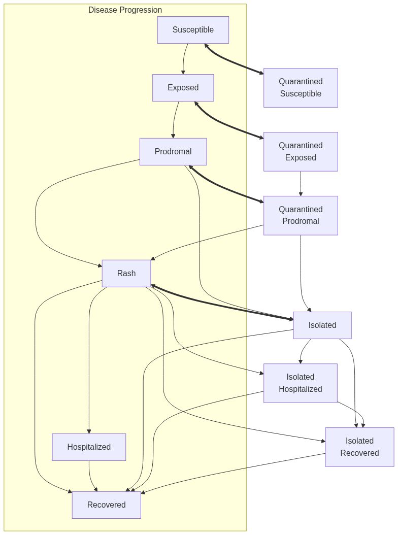
Measles model with mixing
Description
ModelMeaslesMixing creates a measles epidemiological model with mixing
between different population groups. The model includes vaccination,
quarantine, isolation, and contact tracing mechanisms.
Usage
ModelMeaslesMixing(
  n,
  prevalence,
  contact_matrix,
  vax_reduction_recovery_rate = 0.5,
  transmission_rate = 0.9,
  contact_rate = 15/transmission_rate/prodromal_period,
  prop_vaccinated,
  vax_efficacy = 0.99,
  quarantine_period = 21,
  quarantine_willingness = 1,
  isolation_willingness = 1,
  isolation_period = 4,
  incubation_period = 12,
  prodromal_period = 4,
  rash_period = 3,
  hospitalization_rate = 0.2,
  hospitalization_period = 7,
  days_undetected = 2,
  contact_tracing_success_rate = 1,
  contact_tracing_days_prior = 4
)
Arguments
n |
Number of individuals in the population. |
prevalence |
Double. Initial proportion of individuals with the virus. |
contact_matrix |
A row-stochastic matrix of mixing proportions between population groups. |
vax_reduction_recovery_rate |
Double. Vaccine reduction in recovery rate (default: 0.5). |
transmission_rate |
Numeric scalar between 0 and 1. Probability of transmission (default: 0.9). |
contact_rate |
Numeric scalar. Average number of contacts per step. |
prop_vaccinated |
Double. Proportion of population that is vaccinated. |
vax_efficacy |
Double. Vaccine efficacy rate (default: 0.99). |
quarantine_period |
Integer. Number of days for quarantine (default: 21). |
quarantine_willingness |
Double. Proportion of agents willing to quarantine (default: 1). |
isolation_willingness |
Double. Proportion of agents willing to isolate (default: 1). |
isolation_period |
Integer. Number of days for isolation (default: 4). |
incubation_period |
Double. Duration of incubation period (default: 12). |
prodromal_period |
Double. Duration of prodromal period (default: 4). |
rash_period |
Double. Duration of rash period (default: 3). |
hospitalization_rate |
Double. Rate of hospitalization (default: 0.2). |
hospitalization_period |
Double. Period of hospitalization (default: 7). |
days_undetected |
Double. Number of days an infection goes undetected (default: 2). |
contact_tracing_success_rate |
Double. Probability of successful contact tracing (default: 1.0). |
contact_tracing_days_prior |
Integer. Number of days prior to the onset of the infection for which contact tracing is effective (default: 4). |
Details
The contact_matrix is a matrix of contact rates between entities. The
matrix should be of size n x n, where n is the number of entities.
This is a row-stochastic matrix, i.e., the sum of each row should be 1.
The model includes three distinct phases of measles infection: incubation, prodromal, and rash periods. Vaccination provides protection against infection and may reduce recovery time.
The initial_states function allows the user to set the initial state of the model. In particular, the user can specify how many of the non-infected agents have been removed at the beginning of the simulation.
The default value for the contact rate is an approximation to the disease's basic reproduction number (R0), but it is not 100% accurate. A more accurate way to se the contact rate is available, and will be distributed in the future.
Value
The
ModelMeaslesMixingfunction returns a model of classes epiworld_model and epiworld_measlesmixing.
Model diagram
See Also
epiworld-methods
Other Models:
ModelDiffNet(),
ModelMeaslesMixingRiskQuarantine(),
ModelMeaslesSchool(),
ModelSEIR(),
ModelSEIRCONN(),
ModelSEIRD(),
ModelSEIRDCONN(),
ModelSEIRMixing(),
ModelSEIRMixingQuarantine(),
ModelSIR(),
ModelSIRCONN(),
ModelSIRD(),
ModelSIRDCONN(),
ModelSIRLogit(),
ModelSIRMixing(),
ModelSIS(),
ModelSISD(),
ModelSURV(),
epiworld-data
Other measles models:
ModelMeaslesMixingRiskQuarantine(),
ModelMeaslesSchool()
Examples
# Start off creating three entities.
# Individuals will be distributed randomly between the three.
e1 <- entity("Population 1", 3e3, as_proportion = FALSE)
e2 <- entity("Population 2", 3e3, as_proportion = FALSE)
e3 <- entity("Population 3", 3e3, as_proportion = FALSE)

# Row-stochastic matrix (rowsums 1)
cmatrix <- c(
  c(0.9, 0.05, 0.05),
  c(0.1, 0.8, 0.1),
  c(0.1, 0.2, 0.7)
) |> matrix(byrow = TRUE, nrow = 3)

N <- 9e3

measles_model <- ModelMeaslesMixing(
  n                        = N,
  prevalence               = 1 / N,
  contact_rate             = 15,
  transmission_rate        = 0.9,
  vax_efficacy             = 0.97,
  vax_reduction_recovery_rate = 0.8,
  incubation_period        = 10,
  prodromal_period         = 3,
  rash_period              = 7,
  contact_matrix           = cmatrix,
  hospitalization_rate     = 0.1,
  hospitalization_period   = 10,
  days_undetected          = 2,
  quarantine_period        = 14,
  quarantine_willingness   = 0.9,
  isolation_willingness    = 0.8,
  isolation_period         = 10,
  prop_vaccinated          = 0.95,
  contact_tracing_success_rate = 0.8,
  contact_tracing_days_prior = 4
)

# Adding the entities to the model
measles_model |>
  add_entity(e1) |>
  add_entity(e2) |>
  add_entity(e3)

set.seed(331)
run(measles_model, ndays = 100)
summary(measles_model)
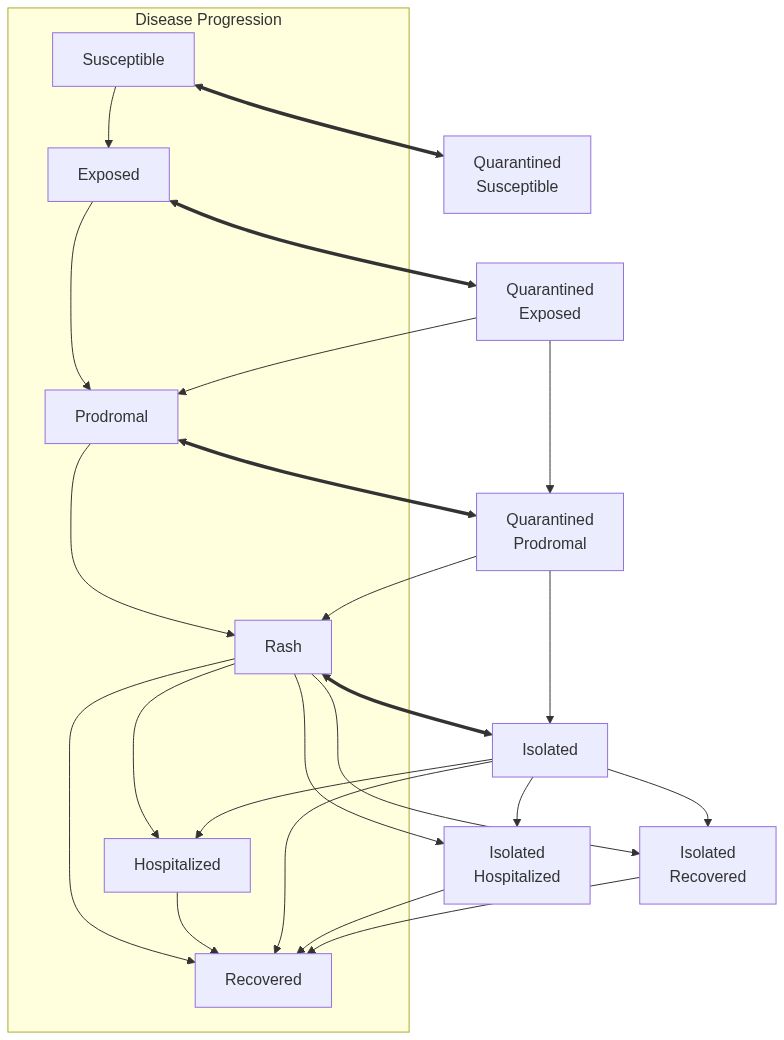
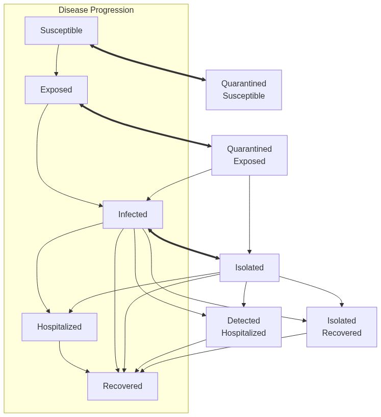
Measles model with mixing and risk-based quarantine
Description
ModelMeaslesMixingRiskQuarantine creates a measles epidemiological model with mixing
between different population groups and risk-based quarantine strategies. The model
includes vaccination, quarantine with three risk levels (high, medium, low), isolation,
and contact tracing mechanisms.
Usage
ModelMeaslesMixingRiskQuarantine(
  n,
  prevalence,
  contact_matrix,
  transmission_rate = 0.9,
  contact_rate = 15/transmission_rate/prodromal_period,
  prop_vaccinated,
  vax_efficacy = 0.99,
  quarantine_period_high = 21,
  quarantine_period_medium = 14,
  quarantine_period_low = 7,
  quarantine_willingness = 1,
  isolation_willingness = 1,
  isolation_period = 4,
  incubation_period = 12,
  prodromal_period = 4,
  rash_period = 3,
  hospitalization_rate = 0.2,
  hospitalization_period = 7,
  days_undetected = 2,
  detection_rate_quarantine = 0.5,
  contact_tracing_success_rate = 1,
  contact_tracing_days_prior = 4
)
Arguments
n |
Number of individuals in the population. |
prevalence |
Double. Initial proportion of individuals with the virus. |
contact_matrix |
A row-stochastic matrix of mixing proportions between population groups. |
transmission_rate |
Numeric scalar between 0 and 1. Probability of transmission (default: 0.9). |
contact_rate |
Numeric scalar. Average number of contacts per step. |
prop_vaccinated |
Double. Proportion of population that is vaccinated. |
vax_efficacy |
Double. Vaccine efficacy rate (default: 0.99). |
quarantine_period_high |
Integer. Number of days for quarantine for high-risk contacts (default: 21). |
quarantine_period_medium |
Integer. Number of days for quarantine for medium-risk contacts (default: 14). |
quarantine_period_low |
Integer. Number of days for quarantine for low-risk contacts (default: 7). |
quarantine_willingness |
Double. Proportion of agents willing to quarantine (default: 1). |
isolation_willingness |
Double. Proportion of agents willing to isolate (default: 1). |
isolation_period |
Integer. Number of days for isolation (default: 4). |
incubation_period |
Double. Duration of incubation period (default: 12). |
prodromal_period |
Double. Duration of prodromal period (default: 4). |
rash_period |
Double. Duration of rash period (default: 3). |
hospitalization_rate |
Double. Rate of hospitalization (default: 0.2). |
hospitalization_period |
Double. Period of hospitalization (default: 7). |
days_undetected |
Double. Number of days rash goes undetected (default: 2). |
detection_rate_quarantine |
Double. Detection rate of prodromal agents during active quarantine periods (default: 0.5). |
contact_tracing_success_rate |
Double. Probability of successful contact tracing (default: 1.0). |
contact_tracing_days_prior |
Integer. Number of days prior to the onset of the infection for which contact tracing is effective (default: 4). |
Details
The contact_matrix is a matrix of contact rates between entities. The
matrix should be of size n x n, where n is the number of entities.
This is a row-stochastic matrix, i.e., the sum of each row should be 1.
The model includes three distinct phases of measles infection: incubation (exposed), prodromal, and rash periods. Vaccination provides protection against transmission.
Risk-based quarantine strategies assign different quarantine durations based on exposure risk:
-
High Risk: Unvaccinated agents who share entity membership with the case
-
Medium Risk: Unvaccinated agents who contacted an infected individual but don't share entity membership
-
Low Risk: Other unvaccinated agents
The initial_states function allows the user to set the initial state of the model. In particular, the user can specify how many of the non-infected agents have been removed at the beginning of the simulation.
The default value for the contact rate is an approximation to the disease's basic reproduction number (R0), but it is not 100% accurate. A more accurate way to set the contact rate is available, and will be distributed in the future.
Value
The
ModelMeaslesMixingRiskQuarantinefunction returns a model of classes epiworld_model and epiworld_measlesmixingriskquarantine.
Model diagram
See Also
epiworld-methods
Other Models:
ModelDiffNet(),
ModelMeaslesMixing(),
ModelMeaslesSchool(),
ModelSEIR(),
ModelSEIRCONN(),
ModelSEIRD(),
ModelSEIRDCONN(),
ModelSEIRMixing(),
ModelSEIRMixingQuarantine(),
ModelSIR(),
ModelSIRCONN(),
ModelSIRD(),
ModelSIRDCONN(),
ModelSIRLogit(),
ModelSIRMixing(),
ModelSIS(),
ModelSISD(),
ModelSURV(),
epiworld-data
Other measles models:
ModelMeaslesMixing(),
ModelMeaslesSchool()
Examples
# Start off creating three entities.
# Individuals will be distributed randomly between the three.
e1 <- entity("Population 1", 3e3, as_proportion = FALSE)
e2 <- entity("Population 2", 3e3, as_proportion = FALSE)
e3 <- entity("Population 3", 3e3, as_proportion = FALSE)

# Row-stochastic matrix (rowsums 1)
cmatrix <- c(
  c(0.9, 0.05, 0.05),
  c(0.1, 0.8, 0.1),
  c(0.1, 0.2, 0.7)
) |> matrix(byrow = TRUE, nrow = 3)

N <- 9e3

measles_model <- ModelMeaslesMixingRiskQuarantine(
  n                        = N,
  prevalence               = 1 / N,
  contact_rate             = 15,
  transmission_rate        = 0.9,
  vax_efficacy             = 0.97,
  incubation_period        = 10,
  prodromal_period         = 3,
  rash_period              = 7,
  contact_matrix           = cmatrix,
  hospitalization_rate     = 0.1,
  hospitalization_period   = 10,
  days_undetected          = 2,
  quarantine_period_high   = 21,
  quarantine_period_medium = 14,
  quarantine_period_low    = 7,
  quarantine_willingness   = 0.9,
  isolation_willingness    = 0.8,
  isolation_period         = 10,
  prop_vaccinated          = 0.95,
  detection_rate_quarantine = 0.5,
  contact_tracing_success_rate = 0.8,
  contact_tracing_days_prior = 4
)

# Adding the entities to the model
measles_model |>
  add_entity(e1) |>
  add_entity(e2) |>
  add_entity(e3)

set.seed(331)
run(measles_model, ndays = 100)
summary(measles_model)
Deprecated and removed functions in epiworldR
Description
Starting version 0.0-4, epiworld changed how it refered to "actions." Following more traditional ABMs, actions are now called "events."
Usage
ModelMeaslesQuarantine(...)

add_tool_n(model, tool, n)

add_virus_n(model, virus, n)

globalaction_tool(...)

globalaction_tool_logit(...)

globalaction_set_params(...)

globalaction_fun(...)
Arguments
... |
Arguments to be passed to the new function. |
model |
Model object of class |
tool |
Tool object of class |
n |
Deprecated. |
virus |
Virus object of class |
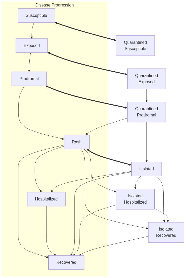
Measles model with quarantine
Description
Implements a Susceptible-Exposed-Infectious-Hospitalized-Recovered (SEIHR) model for Measles within a school. The model includes isolation of detected cases and optional quarantine of unvaccinated individuals.
Usage
ModelMeaslesSchool(
  n,
  prevalence = 1,
  contact_rate = 15/transmission_rate/prodromal_period,
  transmission_rate = 0.9,
  vax_efficacy = 0.99,
  incubation_period = 12,
  prodromal_period = 4,
  rash_period = 3,
  days_undetected = 2,
  hospitalization_rate = 0.2,
  hospitalization_period = 7,
  prop_vaccinated = 1 - 1/15,
  quarantine_period = 21,
  quarantine_willingness = 1,
  isolation_period = 4,
  ...
)
Arguments
n |
Number of agents in the model. |
prevalence |
Initial number of agents with the virus. |
contact_rate |
Average number of contacts per step. Default is set to match the basic reproductive number (R0) of 15 (see details). |
transmission_rate |
Probability of transmission. |
vax_efficacy |
Probability of vaccine efficacy. |
incubation_period |
Average number of incubation days. |
prodromal_period |
Average number of prodromal days. |
rash_period |
Average number of rash days. |
days_undetected |
Average number of days undetected. Detected cases are moved to isolation and trigger the quarantine process. |
hospitalization_rate |
Probability of hospitalization. |
hospitalization_period |
Average number of days in hospital. |
prop_vaccinated |
Proportion of the population vaccinated. |
quarantine_period |
Number of days an agent is in quarantine. |
quarantine_willingness |
Probability of accepting quarantine ( see details). |
isolation_period |
Number of days an agent is in isolation. |
... |
Further arguments (not used). |
Details
This model can be described as a SEIHR model with isolation and quarantine. The infectious state is divided into prodromal and rash phases. Furthermore, the quarantine state includes exposed, susceptible, prodromal, and recovered states.
The model is a perfect mixing model, meaning that all agents are in contact with each other. The model is designed to simulate the spread of Measles within a school setting, where the population is assumed to be homogeneous.
The quarantine process is triggered any time that an agent with rash is
detected. The agent is then isolated and all agents who are unvaccinated are
quarantined (if willing). Isolated agents then may be moved out of the
isolation in isolation_period days. The quarantine willingness parameter
sets the probability of accepting quarantine. If a quarantined agent develops
rash, they are moved to isolation, which triggers a new quarantine process.
The basic reproductive number in Measles is estimated to be about 15. By default, the contact rate of the model is set so that the R0 matches 15.
When quarantine_period is set to -1, the model assumes
there is no quarantine process. The same happens with isolation_period.
Since the quarantine process is triggered by an isolation, then
isolation_period = -1 automatically sets quarantine_period = -1.
Value
The
ModelMeaslesQuarantinefunction returns a model of classes epiworld_model andepiworld_measlesquarantine.
Model diagram
Note
As of version 0.10.0, the parameter vax_improved_recovery has been removed
and is no longer used (it never had a side effect). Future versions may not
accept it.
Author(s)
This model was built as a response to the US Measles outbreak in 2025. This is a collaboration between the University of Utah (ForeSITE center grant) and the Utah Department of Health and Human Services.
References
Jones, Trahern W, and Katherine Baranowski. 2019. "Measles and Mumps: Old Diseases, New Outbreaks."
Liu, Fengchen, Wayne T A Enanoria, Jennifer Zipprich, Seth Blumberg, Kathleen Harriman, Sarah F Ackley, William D Wheaton, Justine L Allpress, and Travis C Porco. 2015. "The Role of Vaccination Coverage, Individual Behaviors, and the Public Health Response in the Control of Measles Epidemics: An Agent-Based Simulation for California." BMC Public Health 15 (1): 447. doi:10.1186/s12889-015-1766-6.
"Measles Disease Plan." 2019. Utah Department of Health and Human Services. https://epi.utah.gov/wp-content/uploads/Measles-disease-plan.pdf.
See Also
epiworld-methods
Other Models:
ModelDiffNet(),
ModelMeaslesMixing(),
ModelMeaslesMixingRiskQuarantine(),
ModelSEIR(),
ModelSEIRCONN(),
ModelSEIRD(),
ModelSEIRDCONN(),
ModelSEIRMixing(),
ModelSEIRMixingQuarantine(),
ModelSIR(),
ModelSIRCONN(),
ModelSIRD(),
ModelSIRDCONN(),
ModelSIRLogit(),
ModelSIRMixing(),
ModelSIS(),
ModelSISD(),
ModelSURV(),
epiworld-data
Other measles models:
ModelMeaslesMixing(),
ModelMeaslesMixingRiskQuarantine()
Examples
# An in a school with low vaccination
model_measles <- ModelMeaslesQuarantine(
  n = 500,
  prevalence = 1,
  prop_vaccinated = 0.70
)

# Running and printing
run(model_measles, ndays = 100, seed = 1912)
model_measles

plot(model_measles)
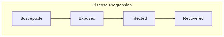
Susceptible Exposed Infected Recovered model (SEIR)
Description
Susceptible Exposed Infected Recovered model (SEIR)
Usage
ModelSEIR(name, prevalence, transmission_rate, incubation_days, recovery_rate)
Arguments
name |
String. Name of the virus. |
prevalence |
Double. Initial proportion of individuals with the virus. |
transmission_rate |
Numeric scalar between 0 and 1. Virus's rate of infection. |
incubation_days |
Numeric scalar greater than 0. Average number of incubation days. |
recovery_rate |
Numeric scalar between 0 and 1. Rate of recovery_rate from virus. |
Details
The initial_states function allows the user to set the initial state of the model. The user must provide a vector of proportions indicating the following values: (1) Proportion of non-infected agents who are removed, and (2) Proportion of exposed agents to be set as infected.
Value
The
ModelSEIRfunction returns a model of class epiworld_model.
Model diagram

See Also
epiworld-methods
Other Models:
ModelDiffNet(),
ModelMeaslesMixing(),
ModelMeaslesMixingRiskQuarantine(),
ModelMeaslesSchool(),
ModelSEIRCONN(),
ModelSEIRD(),
ModelSEIRDCONN(),
ModelSEIRMixing(),
ModelSEIRMixingQuarantine(),
ModelSIR(),
ModelSIRCONN(),
ModelSIRD(),
ModelSIRDCONN(),
ModelSIRLogit(),
ModelSIRMixing(),
ModelSIS(),
ModelSISD(),
ModelSURV(),
epiworld-data
Examples
model_seir <- ModelSEIR(name = "COVID-19", prevalence = 0.01,
  transmission_rate = 0.9, recovery_rate = 0.1, incubation_days = 4)

# Adding a small world population
agents_smallworld(
  model_seir,
  n = 1000,
  k = 5,
  d = FALSE,
  p = .01
)

# Running and printing
run(model_seir, ndays = 100, seed = 1912)
model_seir

plot(model_seir, main = "SEIR Model")
Susceptible Exposed Infected Removed model (SEIR connected)
Description
The SEIR connected model implements a model where all agents are connected. This is equivalent to a compartmental model (wiki).
Usage
ModelSEIRCONN(
  name,
  n,
  prevalence,
  contact_rate,
  transmission_rate,
  incubation_days,
  recovery_rate
)
Arguments
name |
String. Name of the virus. |
n |
Number of individuals in the population. |
prevalence |
Initial proportion of individuals with the virus. |
contact_rate |
Numeric scalar. Average number of contacts per step. |
transmission_rate |
Numeric scalar between 0 and 1. Probability of transmission. |
incubation_days |
Numeric scalar greater than 0. Average number of incubation days. |
recovery_rate |
Numeric scalar between 0 and 1. Probability of recovery_rate. |
Value
The
ModelSEIRCONNfunction returns a model of class epiworld_model.
Model diagram
See Also
epiworld-methods
Other Models:
ModelDiffNet(),
ModelMeaslesMixing(),
ModelMeaslesMixingRiskQuarantine(),
ModelMeaslesSchool(),
ModelSEIR(),
ModelSEIRD(),
ModelSEIRDCONN(),
ModelSEIRMixing(),
ModelSEIRMixingQuarantine(),
ModelSIR(),
ModelSIRCONN(),
ModelSIRD(),
ModelSIRDCONN(),
ModelSIRLogit(),
ModelSIRMixing(),
ModelSIS(),
ModelSISD(),
ModelSURV(),
epiworld-data
Examples
# An example with COVID-19
model_seirconn <- ModelSEIRCONN(
  name                = "COVID-19",
  prevalence          = 0.01,
  n                   = 10000,
  contact_rate        = 2,
  incubation_days     = 7,
  transmission_rate   = 0.5,
  recovery_rate       = 0.3
)

# Running and printing
run(model_seirconn, ndays = 100, seed = 1912)
model_seirconn

plot(model_seirconn)

# Adding the flu
flu <- virus("Flu", .9, 1 / 7, prevalence = 0.001, as_proportion = TRUE)
add_virus(model_seirconn, flu)

#' # Running and printing
run(model_seirconn, ndays = 100, seed = 1912)
model_seirconn

plot(model_seirconn)
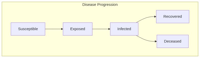
Susceptible-Exposed-Infected-Recovered-Deceased model (SEIRD)
Description
Susceptible-Exposed-Infected-Recovered-Deceased model (SEIRD)
Usage
ModelSEIRD(
  name,
  prevalence,
  transmission_rate,
  incubation_days,
  recovery_rate,
  death_rate
)
Arguments
name |
String. Name of the virus. |
prevalence |
Double. Initial proportion of individuals with the virus. |
transmission_rate |
Numeric scalar between 0 and 1. Virus's rate of infection. |
incubation_days |
Numeric scalar greater than 0. Average number of incubation days. |
recovery_rate |
Numeric scalar between 0 and 1. Rate of recovery_rate from virus. |
death_rate |
Numeric scalar between 0 and 1. Rate of death from virus. |
Details
The initial_states function allows the user to set the initial state of the model. The user must provide a vector of proportions indicating the following values: (1) Proportion of exposed agents who are infected, (2) proportion of non-infected agents already removed, and (3) proportion of non-ifected agents already deceased.
Value
The
ModelSEIRDfunction returns a model of class epiworld_model.
Model diagram
See Also
epiworld-methods
Other Models:
ModelDiffNet(),
ModelMeaslesMixing(),
ModelMeaslesMixingRiskQuarantine(),
ModelMeaslesSchool(),
ModelSEIR(),
ModelSEIRCONN(),
ModelSEIRDCONN(),
ModelSEIRMixing(),
ModelSEIRMixingQuarantine(),
ModelSIR(),
ModelSIRCONN(),
ModelSIRD(),
ModelSIRDCONN(),
ModelSIRLogit(),
ModelSIRMixing(),
ModelSIS(),
ModelSISD(),
ModelSURV(),
epiworld-data
Examples
model_seird <- ModelSEIRD(name = "COVID-19", prevalence = 0.01,
  transmission_rate = 0.9, recovery_rate = 0.1, incubation_days = 4,
  death_rate = 0.01)

# Adding a small world population
agents_smallworld(
  model_seird,
  n = 100000,
  k = 5,
  d = FALSE,
  p = .01
)

# Running and printing
run(model_seird, ndays = 100, seed = 1912)
model_seird

plot(model_seird, main = "SEIRD Model")
Susceptible Exposed Infected Removed Deceased model (SEIRD connected)
Description
The SEIRD connected model implements a model where all agents are connected. This is equivalent to a compartmental model (wiki).
Usage
ModelSEIRDCONN(
  name,
  n,
  prevalence,
  contact_rate,
  transmission_rate,
  incubation_days,
  recovery_rate,
  death_rate
)
Arguments
name |
String. Name of the virus. |
n |
Number of individuals in the population. |
prevalence |
Initial proportion of individuals with the virus. |
contact_rate |
Numeric scalar. Average number of contacts per step. |
transmission_rate |
Numeric scalar between 0 and 1. Probability of transmission. |
incubation_days |
Numeric scalar greater than 0. Average number of incubation days. |
recovery_rate |
Numeric scalar between 0 and 1. Probability of recovery_rate. |
death_rate |
Numeric scalar between 0 and 1. Probability of death. |
Details
The initial_states function allows the user to set the initial state of the model. The user must provide a vector of proportions indicating the following values: (1) Proportion of exposed agents who are infected, (2) proportion of non-infected agents already removed, and (3) proportion of non-ifected agents already deceased.
Value
The
ModelSEIRDCONNfunction returns a model of class epiworld_model.
Model diagram

See Also
epiworld-methods
Other Models:
ModelDiffNet(),
ModelMeaslesMixing(),
ModelMeaslesMixingRiskQuarantine(),
ModelMeaslesSchool(),
ModelSEIR(),
ModelSEIRCONN(),
ModelSEIRD(),
ModelSEIRMixing(),
ModelSEIRMixingQuarantine(),
ModelSIR(),
ModelSIRCONN(),
ModelSIRD(),
ModelSIRDCONN(),
ModelSIRLogit(),
ModelSIRMixing(),
ModelSIS(),
ModelSISD(),
ModelSURV(),
epiworld-data
Examples
# An example with COVID-19
model_seirdconn <- ModelSEIRDCONN(
  name                = "COVID-19",
  prevalence          = 0.01,
  n                   = 10000,
  contact_rate        = 2,
  incubation_days     = 7,
  transmission_rate   = 0.5,
  recovery_rate       = 0.3,
  death_rate          = 0.01
)

# Running and printing
run(model_seirdconn, ndays = 100, seed = 1912)
model_seirdconn

plot(model_seirdconn)

# Adding the flu
flu <- virus(
  "Flu", prob_infecting = .3, recovery_rate = 1 / 7,
  prob_death = 0.001,
  prevalence = 0.001, as_proportion = TRUE
)
add_virus(model = model_seirdconn, virus = flu)

#' # Running and printing
run(model_seirdconn, ndays = 100, seed = 1912)
model_seirdconn

plot(model_seirdconn)
Susceptible Exposed Infected Removed model (SEIR) with mixing
Description
Susceptible Exposed Infected Removed model (SEIR) with mixing
Usage
ModelSEIRMixing(
  name,
  n,
  prevalence,
  contact_rate,
  transmission_rate,
  incubation_days,
  recovery_rate,
  contact_matrix
)
Arguments
name |
String. Name of the virus |
n |
Number of individuals in the population. |
prevalence |
Double. Initial proportion of individuals with the virus. |
contact_rate |
Numeric scalar. Average number of contacts per step. |
transmission_rate |
Numeric scalar between 0 and 1. Probability of transmission. |
incubation_days |
Numeric scalar. Average number of days in the incubation period. |
recovery_rate |
Numeric scalar between 0 and 1. Probability of recovery. |
contact_matrix |
Matrix of contact rates between individuals. |
Details
The contact_matrix is a matrix of contact rates between entities. The
matrix should be of size n x n, where n is the number of entities.
This is a row-stochastic matrix, i.e., the sum of each row should be 1.
The initial_states function allows the user to set the initial state of the model. In particular, the user can specify how many of the non-infected agents have been removed at the beginning of the simulation.
Value
The
ModelSEIRMixingfunction returns a model of class epiworld_model.
Model diagram

See Also
epiworld-methods
Other Models:
ModelDiffNet(),
ModelMeaslesMixing(),
ModelMeaslesMixingRiskQuarantine(),
ModelMeaslesSchool(),
ModelSEIR(),
ModelSEIRCONN(),
ModelSEIRD(),
ModelSEIRDCONN(),
ModelSEIRMixingQuarantine(),
ModelSIR(),
ModelSIRCONN(),
ModelSIRD(),
ModelSIRDCONN(),
ModelSIRLogit(),
ModelSIRMixing(),
ModelSIS(),
ModelSISD(),
ModelSURV(),
epiworld-data
Examples
# Start off creating three entities.
# Individuals will be distribured randomly between the three.
e1 <- entity("Population 1", 3e3, as_proportion = FALSE)
e2 <- entity("Population 2", 3e3, as_proportion = FALSE)
e3 <- entity("Population 3", 3e3, as_proportion = FALSE)

# Row-stochastic matrix (rowsums 1)
cmatrix <- c(
  c(0.9, 0.05, 0.05),
  c(0.1, 0.8, 0.1),
  c(0.1, 0.2, 0.7)
) |> matrix(byrow = TRUE, nrow = 3)

N <- 9e3

flu_model <- ModelSEIRMixing(
  name              = "Flu",
  n                 = N,
  prevalence        = 1 / N,
  contact_rate      = 20,
  transmission_rate = 0.1,
  recovery_rate     = 1 / 7,
  incubation_days   = 7,
  contact_matrix    = cmatrix
)

# Adding the entities to the model
flu_model |>
  add_entity(e1) |>
  add_entity(e2) |>
  add_entity(e3)

set.seed(331)
run(flu_model, ndays = 100)
summary(flu_model)
plot_incidence(flu_model)
Susceptible Exposed Infected Removed model (SEIR) with mixing and quarantine
Description
ModelSEIRMixingQuarantine creates a model of the SEIR type with mixing and
a quarantine mechanism. Agents who are infected can be quarantined or
isolated. Isolation happens after the agent has been detected as infected,
and agents who have been in contact with the detected person will me moved
to quarantined status.
Usage
ModelSEIRMixingQuarantine(
  name,
  n,
  prevalence,
  contact_rate,
  transmission_rate,
  incubation_days,
  recovery_rate,
  contact_matrix,
  hospitalization_rate,
  hospitalization_period,
  days_undetected,
  quarantine_period,
  quarantine_willingness,
  isolation_willingness,
  isolation_period,
  contact_tracing_success_rate,
  contact_tracing_days_prior
)
Arguments
name |
String. Name of the virus |
n |
Number of individuals in the population. |
prevalence |
Double. Initial proportion of individuals with the virus. |
contact_rate |
Numeric scalar. Average number of contacts per step. |
transmission_rate |
Numeric scalar between 0 and 1. Probability of transmission. |
incubation_days |
Numeric scalar. Average number of days in the incubation period. |
recovery_rate |
Numeric scalar between 0 and 1. Probability of recovery. |
contact_matrix |
Matrix of contact rates between individuals. |
hospitalization_rate |
Double. Rate of hospitalization. |
hospitalization_period |
Double. Period of hospitalization. |
days_undetected |
Double. Number of days an infection goes undetected. |
quarantine_period |
Integer. Number of days for quarantine. |
quarantine_willingness |
Double. Proportion of agents willing to quarantine. |
isolation_willingness |
Double. Proportion of agents willing to isolate. |
isolation_period |
Integer. Number of days for isolation. |
contact_tracing_success_rate |
Double. Probability of successful contact tracing. |
contact_tracing_days_prior |
Integer. Number of days prior to the onset of the infection for which contact tracing is effective. |
Details
The contact_matrix is a matrix of contact rates between entities. The
matrix should be of size n x n, where n is the number of entities.
This is a row-stochastic matrix, i.e., the sum of each row should be 1.
The initial_states function allows the user to set the initial state of the model. In particular, the user can specify how many of the non-infected agents have been removed at the beginning of the simulation.
Value
The
ModelSEIRMixingQuarantinefunction returns a model of class epiworld_model.
Model diagram
See Also
epiworld-methods
Other Models:
ModelDiffNet(),
ModelMeaslesMixing(),
ModelMeaslesMixingRiskQuarantine(),
ModelMeaslesSchool(),
ModelSEIR(),
ModelSEIRCONN(),
ModelSEIRD(),
ModelSEIRDCONN(),
ModelSEIRMixing(),
ModelSIR(),
ModelSIRCONN(),
ModelSIRD(),
ModelSIRDCONN(),
ModelSIRLogit(),
ModelSIRMixing(),
ModelSIS(),
ModelSISD(),
ModelSURV(),
epiworld-data
Examples
# Start off creating three entities.
# Individuals will be distributed randomly between the three.
e1 <- entity("Population 1", 3e3, as_proportion = FALSE)
e2 <- entity("Population 2", 3e3, as_proportion = FALSE)
e3 <- entity("Population 3", 3e3, as_proportion = FALSE)

# Row-stochastic matrix (rowsums 1)
cmatrix <- c(
  c(0.9, 0.05, 0.05),
  c(0.1, 0.8, 0.1),
  c(0.1, 0.2, 0.7)
) |> matrix(byrow = TRUE, nrow = 3)

N <- 9e3

flu_model <- ModelSEIRMixingQuarantine(
  name                  = "Flu",
  n                     = N,
  prevalence            = 1 / N,
  contact_rate          = 20,
  transmission_rate     = 0.1,
  recovery_rate         = 1 / 7,
  incubation_days       = 7,
  contact_matrix        = cmatrix,
  hospitalization_rate  = 0.05,
  hospitalization_period = 7,
  days_undetected       = 3,
  quarantine_period     = 14,
  quarantine_willingness = 0.8,
  isolation_period      = 7,
  isolation_willingness = 0.5,
  contact_tracing_success_rate = 0.7,
  contact_tracing_days_prior = 3
)

# Adding the entities to the model
flu_model |>
  add_entity(e1) |>
  add_entity(e2) |>
  add_entity(e3)

set.seed(331)
run(flu_model, ndays = 100)
summary(flu_model)
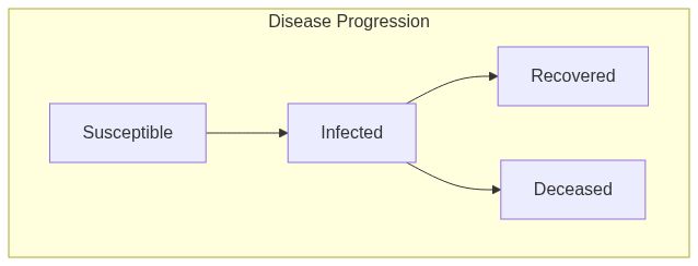
SIR model
Description
SIR model
Usage
ModelSIR(name, prevalence, transmission_rate, recovery_rate)
Arguments
name |
String. Name of the virus |
prevalence |
Double. Initial proportion of individuals with the virus. |
transmission_rate |
Numeric scalar between 0 and 1. Virus's rate of infection. |
recovery_rate |
Numeric scalar between 0 and 1. Rate of recovery_rate from virus. |
Details
The initial_states function allows the user to set the initial state of the model. In particular, the user can specify how many of the non-infected agents have been removed at the beginning of the simulation.
Value
The
ModelSIRfunction returns a model of class epiworld_model.
Model diagram

See Also
epiworld-methods
Other Models:
ModelDiffNet(),
ModelMeaslesMixing(),
ModelMeaslesMixingRiskQuarantine(),
ModelMeaslesSchool(),
ModelSEIR(),
ModelSEIRCONN(),
ModelSEIRD(),
ModelSEIRDCONN(),
ModelSEIRMixing(),
ModelSEIRMixingQuarantine(),
ModelSIRCONN(),
ModelSIRD(),
ModelSIRDCONN(),
ModelSIRLogit(),
ModelSIRMixing(),
ModelSIS(),
ModelSISD(),
ModelSURV(),
epiworld-data
Examples
model_sir <- ModelSIR(name = "COVID-19", prevalence = 0.01,
  transmission_rate = 0.9, recovery_rate = 0.1)

# Adding a small world population
agents_smallworld(
  model_sir,
  n = 1000,
  k = 5,
  d = FALSE,
  p = .01
)

# Running and printing
run(model_sir, ndays = 100, seed = 1912)
model_sir

# Plotting
plot(model_sir)
Susceptible Infected Removed model (SIR connected)
Description
Susceptible Infected Removed model (SIR connected)
Usage
ModelSIRCONN(
  name,
  n,
  prevalence,
  contact_rate,
  transmission_rate,
  recovery_rate
)
Arguments
name |
String. Name of the virus |
n |
Number of individuals in the population. |
prevalence |
Double. Initial proportion of individuals with the virus. |
contact_rate |
Numeric scalar. Average number of contacts per step. |
transmission_rate |
Numeric scalar between 0 and 1. Probability of transmission. |
recovery_rate |
Numeric scalar between 0 and 1. Probability of recovery. |
Details
The initial_states function allows the user to set the initial state of the model. In particular, the user can specify how many of the non-infected agents have been removed at the beginning of the simulation.
Value
The
ModelSIRCONNfunction returns a model of class epiworld_model.
Model diagram

See Also
epiworld-methods
Other Models:
ModelDiffNet(),
ModelMeaslesMixing(),
ModelMeaslesMixingRiskQuarantine(),
ModelMeaslesSchool(),
ModelSEIR(),
ModelSEIRCONN(),
ModelSEIRD(),
ModelSEIRDCONN(),
ModelSEIRMixing(),
ModelSEIRMixingQuarantine(),
ModelSIR(),
ModelSIRD(),
ModelSIRDCONN(),
ModelSIRLogit(),
ModelSIRMixing(),
ModelSIS(),
ModelSISD(),
ModelSURV(),
epiworld-data
Examples
model_sirconn <- ModelSIRCONN(
  name                = "COVID-19",
  n                   = 10000,
  prevalence          = 0.01,
  contact_rate        = 5,
  transmission_rate   = 0.4,
  recovery_rate       = 0.95
)

# Running and printing
run(model_sirconn, ndays = 100, seed = 1912)
model_sirconn

plot(model_sirconn,  main = "SIRCONN Model")
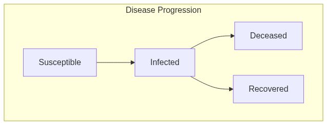
SIRD model
Description
SIRD model
Usage
ModelSIRD(name, prevalence, transmission_rate, recovery_rate, death_rate)
Arguments
name |
String. Name of the virus |
prevalence |
Double. Initial proportion of individuals with the virus. |
transmission_rate |
Numeric scalar between 0 and 1. Virus's rate of infection. |
recovery_rate |
Numeric scalar between 0 and 1. Rate of recovery_rate from virus. |
death_rate |
Numeric scalar between 0 and 1. Rate of death from virus. |
Details
The initial_states function allows the user to set the initial state of the model. The user must provide a vector of proportions indicating the following values: (1) proportion of non-infected agents already removed, and (2) proportion of non-ifected agents already deceased.
Value
The
ModelSIRDfunction returns a model of class epiworld_model.
Model diagram
See Also
epiworld-methods
Other Models:
ModelDiffNet(),
ModelMeaslesMixing(),
ModelMeaslesMixingRiskQuarantine(),
ModelMeaslesSchool(),
ModelSEIR(),
ModelSEIRCONN(),
ModelSEIRD(),
ModelSEIRDCONN(),
ModelSEIRMixing(),
ModelSEIRMixingQuarantine(),
ModelSIR(),
ModelSIRCONN(),
ModelSIRDCONN(),
ModelSIRLogit(),
ModelSIRMixing(),
ModelSIS(),
ModelSISD(),
ModelSURV(),
epiworld-data
Examples
model_sird <- ModelSIRD(
  name              = "COVID-19",
  prevalence        = 0.01,
  transmission_rate = 0.9,
  recovery_rate     = 0.1,
  death_rate        = 0.01
)

# Adding a small world population
agents_smallworld(
  model_sird,
  n = 1000,
  k = 5,
  d = FALSE,
  p = .01
)

# Running and printing
run(model_sird, ndays = 100, seed = 1912)
model_sird

# Plotting
plot(model_sird)
Susceptible Infected Removed Deceased model (SIRD connected)
Description
Susceptible Infected Removed Deceased model (SIRD connected)
Usage
ModelSIRDCONN(
  name,
  n,
  prevalence,
  contact_rate,
  transmission_rate,
  recovery_rate,
  death_rate
)
Arguments
name |
String. Name of the virus |
n |
Number of individuals in the population. |
prevalence |
Double. Initial proportion of individuals with the virus. |
contact_rate |
Numeric scalar. Average number of contacts per step. |
transmission_rate |
Numeric scalar between 0 and 1. Probability of transmission. |
recovery_rate |
Numeric scalar between 0 and 1. Probability of recovery. |
death_rate |
Numeric scalar between 0 and 1. Probability of death. |
Details
The initial_states function allows the user to set the initial state of the model. The user must provide a vector of proportions indicating the following values: (1) proportion of non-infected agents already removed, and (2) proportion of non-ifected agents already deceased.
Value
The
ModelSIRDCONNfunction returns a model of class epiworld_model.
Model diagram
See Also
epiworld-methods
Other Models:
ModelDiffNet(),
ModelMeaslesMixing(),
ModelMeaslesMixingRiskQuarantine(),
ModelMeaslesSchool(),
ModelSEIR(),
ModelSEIRCONN(),
ModelSEIRD(),
ModelSEIRDCONN(),
ModelSEIRMixing(),
ModelSEIRMixingQuarantine(),
ModelSIR(),
ModelSIRCONN(),
ModelSIRD(),
ModelSIRLogit(),
ModelSIRMixing(),
ModelSIS(),
ModelSISD(),
ModelSURV(),
epiworld-data
Examples
model_sirdconn <- ModelSIRDCONN(
  name                = "COVID-19",
  n                   = 100000,
  prevalence          = 0.01,
  contact_rate        = 5,
  transmission_rate   = 0.4,
  recovery_rate       = 0.5,
  death_rate          = 0.1
)

# Running and printing
run(model_sirdconn, ndays = 100, seed = 1912)
model_sirdconn

plot(model_sirdconn,  main = "SIRDCONN Model")
SIR Logistic model
Description
SIR Logistic model
Usage
ModelSIRLogit(
  vname,
  data,
  coefs_infect,
  coefs_recover,
  coef_infect_cols,
  coef_recover_cols,
  prob_infection,
  recovery_rate,
  prevalence
)
Arguments
vname |
Name of the virus. |
data |
A numeric matrix with |
coefs_infect |
Numeric vector. Coefficients associated to infect. |
coefs_recover |
Numeric vector. Coefficients associated to recover. |
coef_infect_cols |
Integer vector. Columns in the coeficient. |
coef_recover_cols |
Integer vector. Columns in the coeficient. |
prob_infection |
Numeric scalar. Baseline probability of infection. |
recovery_rate |
Numeric scalar. Baseline probability of recovery. |
prevalence |
Numeric scalar. Prevalence (initial state) in proportion. |
Value
The
ModelSIRLogitfunction returns a model of class epiworld_model.
Model diagram

See Also
Other Models:
ModelDiffNet(),
ModelMeaslesMixing(),
ModelMeaslesMixingRiskQuarantine(),
ModelMeaslesSchool(),
ModelSEIR(),
ModelSEIRCONN(),
ModelSEIRD(),
ModelSEIRDCONN(),
ModelSEIRMixing(),
ModelSEIRMixingQuarantine(),
ModelSIR(),
ModelSIRCONN(),
ModelSIRD(),
ModelSIRDCONN(),
ModelSIRMixing(),
ModelSIS(),
ModelSISD(),
ModelSURV(),
epiworld-data
Examples
set.seed(2223)
n <- 100000

# Creating the data to use for the "ModelSIRLogit" function. It contains
# information on the sex of each agent and will be used to determine
# differences in disease progression between males and females. Note that
# the number of rows in these data are identical to n (100000).
X <- cbind(
  Intercept = 1,
  Female    = sample.int(2, n, replace = TRUE) - 1
)

# Declare coefficients for each sex regarding transmission_rate and recovery.
coef_infect  <- c(.1, -2, 2)
coef_recover <- rnorm(2)

# Feed all above information into the "ModelSIRLogit" function.
model_logit <- ModelSIRLogit(
  "covid2",
  data = X,
  coefs_infect      = coef_infect,
  coefs_recover     = coef_recover,
  coef_infect_cols  = 1L:ncol(X),
  coef_recover_cols = 1L:ncol(X),
  prob_infection = .8,
  recovery_rate = .3,
  prevalence = .01
)

agents_smallworld(model_logit, n, 8, FALSE, .01)

run(model_logit, 50)

plot(model_logit)

# Females are supposed to be more likely to become infected.
rn <- get_reproductive_number(model_logit)

# Probability of infection for males and females.
(table(
  X[, "Female"],
  (1:n %in% rn$source)
) |> prop.table())[, 2]

# Looking into the individual agents.
get_agents(model_logit)
Susceptible Infected Removed model (SIR) with mixing
Description
Susceptible Infected Removed model (SIR) with mixing
Usage
ModelSIRMixing(
  name,
  n,
  prevalence,
  contact_rate,
  transmission_rate,
  recovery_rate,
  contact_matrix
)
Arguments
name |
String. Name of the virus |
n |
Number of individuals in the population. |
prevalence |
Double. Initial proportion of individuals with the virus. |
contact_rate |
Numeric scalar. Average number of contacts per step. |
transmission_rate |
Numeric scalar between 0 and 1. Probability of transmission. |
recovery_rate |
Numeric scalar between 0 and 1. Probability of recovery. |
contact_matrix |
Matrix of contact rates between individuals. |
Details
The contact_matrix is a matrix of contact rates between entities. The
matrix should be of size n x n, where n is the number of entities.
This is a row-stochastic matrix, i.e., the sum of each row should be 1.
The initial_states function allows the user to set the initial state of the model. In particular, the user can specify how many of the non-infected agents have been removed at the beginning of the simulation.
Value
The
ModelSIRMixingfunction returns a model of class epiworld_model.
Model diagram
See Also
epiworld-methods
Other Models:
ModelDiffNet(),
ModelMeaslesMixing(),
ModelMeaslesMixingRiskQuarantine(),
ModelMeaslesSchool(),
ModelSEIR(),
ModelSEIRCONN(),
ModelSEIRD(),
ModelSEIRDCONN(),
ModelSEIRMixing(),
ModelSEIRMixingQuarantine(),
ModelSIR(),
ModelSIRCONN(),
ModelSIRD(),
ModelSIRDCONN(),
ModelSIRLogit(),
ModelSIS(),
ModelSISD(),
ModelSURV(),
epiworld-data
Examples
# From the vignette

# Start off creating three entities.
# Individuals will be distribured randomly between the three.
e1 <- entity("Population 1", 3e3, as_proportion = FALSE)
e2 <- entity("Population 2", 3e3, as_proportion = FALSE)
e3 <- entity("Population 3", 3e3, as_proportion = FALSE)

# Row-stochastic matrix (rowsums 1)
cmatrix <- c(
  c(0.9, 0.05, 0.05),
  c(0.1, 0.8, 0.1),
  c(0.1, 0.2, 0.7)
) |> matrix(byrow = TRUE, nrow = 3)

N <- 9e3

flu_model <- ModelSIRMixing(
  name              = "Flu",
  n                 = N,
  prevalence        = 1 / N,
  contact_rate      = 20,
  transmission_rate = 0.1,
  recovery_rate     = 1 / 7,
  contact_matrix    = cmatrix
)

# Adding the entities to the model
flu_model |>
  add_entity(e1) |>
  add_entity(e2) |>
  add_entity(e3)

set.seed(331)
run(flu_model, ndays = 100)
summary(flu_model)
plot_incidence(flu_model)
SIS model
Description
Susceptible-Infected-Susceptible model (SIS) (wiki)
Usage
ModelSIS(name, prevalence, transmission_rate, recovery_rate)
Arguments
name |
String. Name of the virus. |
prevalence |
Double. Initial proportion of individuals with the virus. |
transmission_rate |
Numeric scalar between 0 and 1. Virus's rate of infection. |
recovery_rate |
Numeric scalar between 0 and 1. Rate of recovery from virus. |
Value
The
ModelSISfunction returns a model of class epiworld_model.
Model diagram
See Also
epiworld-methods
Other Models:
ModelDiffNet(),
ModelMeaslesMixing(),
ModelMeaslesMixingRiskQuarantine(),
ModelMeaslesSchool(),
ModelSEIR(),
ModelSEIRCONN(),
ModelSEIRD(),
ModelSEIRDCONN(),
ModelSEIRMixing(),
ModelSEIRMixingQuarantine(),
ModelSIR(),
ModelSIRCONN(),
ModelSIRD(),
ModelSIRDCONN(),
ModelSIRLogit(),
ModelSIRMixing(),
ModelSISD(),
ModelSURV(),
epiworld-data
Examples
model_sis <- ModelSIS(name = "COVID-19", prevalence = 0.01,
  transmission_rate = 0.9, recovery_rate = 0.1)

# Adding a small world population
agents_smallworld(
  model_sis,
  n = 1000,
  k = 5,
  d = FALSE,
  p = .01
)

# Running and printing
run(model_sis, ndays = 100, seed = 1912)
model_sis

# Plotting
plot(model_sis, main = "SIS Model")
SISD model
Description
Susceptible-Infected-Susceptible-Deceased model (SISD) (wiki)
Usage
ModelSISD(name, prevalence, transmission_rate, recovery_rate, death_rate)
Arguments
name |
String. Name of the virus. |
prevalence |
Double. Initial proportion of individuals with the virus. |
transmission_rate |
Numeric scalar between 0 and 1. Virus's rate of infection. |
recovery_rate |
Numeric scalar between 0 and 1. Rate of recovery from virus. |
death_rate |
Numeric scalar between 0 and 1. Rate of death from virus. |
Value
The
ModelSISDfunction returns a model of class epiworld_model.
Model diagram
See Also
epiworld-methods
Other Models:
ModelDiffNet(),
ModelMeaslesMixing(),
ModelMeaslesMixingRiskQuarantine(),
ModelMeaslesSchool(),
ModelSEIR(),
ModelSEIRCONN(),
ModelSEIRD(),
ModelSEIRDCONN(),
ModelSEIRMixing(),
ModelSEIRMixingQuarantine(),
ModelSIR(),
ModelSIRCONN(),
ModelSIRD(),
ModelSIRDCONN(),
ModelSIRLogit(),
ModelSIRMixing(),
ModelSIS(),
ModelSURV(),
epiworld-data
Examples
model_sisd <- ModelSISD(
  name = "COVID-19",
  prevalence = 0.01,
  transmission_rate = 0.9,
  recovery_rate = 0.1,
  death_rate = 0.01
)

# Adding a small world population
agents_smallworld(
  model_sisd,
  n = 1000,
  k = 5,
  d = FALSE,
  p = .01
)

# Running and printing
run(model_sisd, ndays = 100, seed = 1912)
model_sisd

# Plotting
plot(model_sisd, main = "SISD Model")
SURV model
Description
SURV model
Usage
ModelSURV(
  name,
  prevalence,
  efficacy_vax,
  latent_period,
  infect_period,
  prob_symptoms,
  prop_vaccinated,
  prop_vax_redux_transm,
  prop_vax_redux_infect,
  surveillance_prob,
  transmission_rate,
  prob_death,
  prob_noreinfect
)
Arguments
name |
String. Name of the virus. |
prevalence |
Initial number of individuals with the virus. |
efficacy_vax |
Double. Efficacy of the vaccine. (1 - P(acquire the disease)). |
latent_period |
Double. Shape parameter of a 'Gamma(latent_period, 1)' distribution. This coincides with the expected number of latent days. |
infect_period |
Double. Shape parameter of a 'Gamma(infected_period, 1)' distribution. This coincides with the expected number of infectious days. |
prob_symptoms |
Double. Probability of generating symptoms. |
prop_vaccinated |
Double. Probability of vaccination. Coincides with the initial prevalence of vaccinated individuals. |
prop_vax_redux_transm |
Double. Factor by which the vaccine reduces transmissibility. |
prop_vax_redux_infect |
Double. Factor by which the vaccine reduces the chances of becoming infected. |
surveillance_prob |
Double. Probability of testing an agent. |
transmission_rate |
Double. Raw transmission probability. |
prob_death |
Double. Raw probability of death for symptomatic individuals. |
prob_noreinfect |
Double. Probability of no re-infection. |
Value
The
ModelSURVfunction returns a model of class epiworld_model.
See Also
epiworld-methods
Other Models:
ModelDiffNet(),
ModelMeaslesMixing(),
ModelMeaslesMixingRiskQuarantine(),
ModelMeaslesSchool(),
ModelSEIR(),
ModelSEIRCONN(),
ModelSEIRD(),
ModelSEIRDCONN(),
ModelSEIRMixing(),
ModelSEIRMixingQuarantine(),
ModelSIR(),
ModelSIRCONN(),
ModelSIRD(),
ModelSIRDCONN(),
ModelSIRLogit(),
ModelSIRMixing(),
ModelSIS(),
ModelSISD(),
epiworld-data
Examples
model_surv <- ModelSURV(
  name                  = "COVID-19",
  prevalence            = 20,
  efficacy_vax          = 0.6,
  latent_period         = 4,
  infect_period         = 5,
  prob_symptoms         = 0.5,
  prop_vaccinated       = 0.7,
  prop_vax_redux_transm = 0.8,
  prop_vax_redux_infect = 0.95,
  surveillance_prob     = 0.1,
  transmission_rate     = 0.2,
  prob_death            = 0.001,
  prob_noreinfect       = 0.5
)

# Adding a small world population
agents_smallworld(
  model_surv,
  n = 10000,
  k = 5,
  d = FALSE,
  p = .01
)

# Running and printing
run(model_surv, ndays = 100, seed = 1912)
model_surv

# Plotting
plot(model_surv, main = "SURV Model")
Agents in epiworldR
Description
These functions provide read-access to the agents of the model. The
get_agents function returns an object of class epiworld_agents which
contains all the information about the agents in the model. The
get_agent function returns the information of a single agent.
And the get_state function returns the state of a single agent.
Usage
get_agents(model, ...)

## S3 method for class 'epiworld_model'
get_agents(model, ...)

## S3 method for class 'epiworld_agents'
x[i]

## S3 method for class 'epiworld_agent'
print(x, compressed = FALSE, ...)

## S3 method for class 'epiworld_agents'
print(x, compressed = TRUE, max_print = 10, ...)

get_state(x)
Arguments
model |
An object of class epiworld_model. |
... |
Ignored |
x |
An object of class epiworld_agents |
i |
Index (id) of the agent (from 0 to |
compressed |
Logical scalar. When FALSE, it prints detailed information about the agent. |
max_print |
Integer scalar. Maximum number of agents to print. |
Value
The
get_agentsfunction returns an object of class epiworld_agents.
The
[method returns an object of class epiworld_agent.
The
printfunction returns information about each individual agent of class epiworld_agent.
The
get_statefunction returns the state of the epiworld_agents object.
See Also
agents
Examples
model_sirconn <- ModelSIRCONN(
  name                = "COVID-19",
  n                   = 10000,
  prevalence          = 0.01,
  contact_rate        = 5,
  transmission_rate   = 0.4,
  recovery_rate       = 0.95
)

run(model_sirconn, ndays = 100, seed = 1912)

x <- get_agents(model_sirconn) # Storing all agent information into object of
# class epiworld_agents

print(x, compressed = FALSE, max_print = 5) # Displaying detailed information of
# the first 5 agents using
# compressed=F. Using compressed=T
# results in less-detailed
# information about each agent.

x[0] # Print information about the first agent. Substitute the agent of
# interest's position where '0' is.
Load agents to a model
Description
These functions provide access to the network of the model. The network is
represented by an edgelist. The agents_smallworld function generates a
small world network with the Watts-Strogatz algorithm. The
agents_from_edgelist function loads a network from an edgelist.
The get_network function returns the edgelist of the network.
Usage
agents_smallworld(model, n, k, d, p)

agents_from_edgelist(model, source, target, size, directed)

get_network(model)

get_agents_states(model)

add_virus_agent(agent, model, virus, state_new = -99, queue = -99)

add_tool_agent(agent, model, tool, state_new = -99, queue = -99)

has_virus(agent, virus)

has_tool(agent, tool)

change_state(agent, model, state_new, queue = -99)

get_agents_tools(model)
Arguments
model |
Model object of class epiworld_model. |
n, size |
Number of individuals in the population. |
k |
Number of ties in the small world network. |
d, directed |
Logical scalar. Whether the graph is directed or not. |
p |
Probability of rewiring. |
source, target |
Integer vectors describing the source and target of in the edgelist. |
agent |
Agent object of class |
virus |
Virus object of class |
state_new |
Integer scalar. New state of the agent after the action is executed. |
queue |
Integer scalar. Change in the queuing system after the action is executed. |
tool |
Tool object of class |
Details
The new_state and queue parameters are optional. If they are not
provided, the agent will be updated with the default values of the virus/tool.
Value
The 'agents_smallworld' function returns a model with the agents loaded.
The
agents_from_edgelistfunction returns an empty model of classepiworld_model.
The
get_networkfunction returns a data frame with two columns (sourceandtarget) describing the edgelist of the network.
-
get_agents_statesreturns an character vector with the states of the agents by the end of the simulation.
The function
add_virus_agentadds a virus to an agent and returns the agent invisibly.
The function
add_tool_agentadds a tool to an agent and returns the agent invisibly.
The functions
has_virusandhas_toolreturn a logical scalar indicating whether the agent has the virus/tool or not.
-
get_agents_toolsreturns a list of classepiworld_agents_toolswithepiworld_tools(list of lists).
Examples
# Initializing SIR model with agents_smallworld
sir <- ModelSIR(name = "COVID-19", prevalence = 0.01, transmission_rate = 0.9,
  recovery_rate = 0.1)
agents_smallworld(
  sir,
  n = 1000,
  k = 5,
  d = FALSE,
  p = .01
)
run(sir, ndays = 100, seed = 1912)
sir

# We can also retrieve the network
net <- get_network(sir)
head(net)

# Simulating a bernoulli graph
set.seed(333)
n <- 1000
g <- matrix(runif(n^2) < .01, nrow = n)
diag(g) <- FALSE
el <- which(g, arr.ind = TRUE) - 1L


# Generating an empty model
sir <- ModelSIR("COVID-19", .01, .8, .3)
agents_from_edgelist(
  sir,
  source = el[, 1],
  target = el[, 2],
  size   = n,
  directed = TRUE
)

# Running the simulation
run(sir, 50)

plot(sir)
Get entities
Description
Entities in epiworld are objects that can contain agents.
Usage
get_entities(model)

## S3 method for class 'epiworld_entities'
x[i]

entity(name, prevalence, as_proportion, to_unassigned = TRUE)

get_entity_size(entity)

get_entity_name(entity)

entity_add_agent(entity, agent, model = attr(entity, "model"))

rm_entity(model, id)

add_entity(model, entity)

load_agents_entities_ties(model, agents_id, entities_id)

entity_get_agents(entity)

distribute_entity_randomly(prevalence, as_proportion, to_unassigned = TRUE)

distribute_entity_to_set(agents_ids)

set_distribution_entity(entity, distfun)
Arguments
model |
Model object of class |
x |
Object of class |
i |
Integer index. |
name |
Character scalar. Name of the entity. |
prevalence |
Numeric scalar. Prevalence of the entity. |
as_proportion |
Logical scalar. If |
to_unassigned |
Logical scalar. If |
entity |
Entity object of class |
agent |
Agent object of class |
id |
Integer scalar. Entity id to remove (starting from zero). |
agents_id |
Integer vector. |
entities_id |
Integer vector. |
agents_ids |
Integer vector. Ids of the agents to distribute. |
distfun |
Distribution function object of class |
Details
Epiworld entities are especially useful for mixing models, particularly ModelSIRMixing and ModelSEIRMixing.
Value
The function
entitycreates an entity object.
The function
get_entity_sizereturns the number of agents in the entity.
The function
get_entity_namereturns the name of the entity.
The function
entity_add_agentadds an agent to the entity.
The function
rm_entityremoves an entity from the model.
The function
load_agents_entities_tiesloads agents into entities.
The function
entity_get_agentsreturns an integer vector with the agents in the entity (ids).
Examples
# Creating a mixing model
mymodel <- ModelSIRMixing(
  name = "My model",
  n = 10000,
  prevalence = .001,
  contact_rate = 10,
  transmission_rate = .1,
  recovery_rate = 1 / 7,
  contact_matrix = matrix(c(.9, .1, .1, .9), 2, 2)
)

ent1 <- entity("First", 5000, FALSE)
ent2 <- entity("Second", 5000, FALSE)

mymodel |>
  add_entity(ent1) |>
  add_entity(ent2)

run(mymodel, ndays = 100, seed = 1912)

summary(mymodel)
Accessing the database of epiworld
Description
Models in epiworld are stored in a database. This database can be accessed
using the functions described in this manual page. Some elements of the
database are: the transition matrix, the incidence matrix, the reproductive
number, the generation time, and daily incidence at the virus and tool level.
Usage
get_hist_total(x)

get_today_total(x)

get_hist_virus(x)

get_hist_tool(x)

get_transition_probability(x)

get_reproductive_number(x)

## S3 method for class 'epiworld_repnum'
plot(
  x,
  y = NULL,
  ylab = "Average Rep. Number",
  xlab = "Day (step)",
  main = "Reproductive Number",
  type = "b",
  plot = TRUE,
  ...
)

plot_reproductive_number(x, ...)

get_hist_transition_matrix(x, skip_zeros = FALSE)

## S3 method for class 'epiworld_hist_transition'
as.array(x, ...)

plot_incidence(x, ...)

## S3 method for class 'epiworld_hist_transition'
plot(
  x,
  type = "b",
  xlab = "Day (step)",
  ylab = "Counts",
  main = "Daily incidence",
  plot = TRUE,
  ...
)

get_transmissions(x)

get_generation_time(x)

## S3 method for class 'epiworld_generation_time'
plot(
  x,
  type = "b",
  xlab = "Day (step)",
  ylab = "Avg. Generation Time",
  main = "Generation Time",
  plot = TRUE,
  ...
)

plot_generation_time(x, ...)
Arguments
x |
An object of class |
y |
Ignored. |
ylab, xlab, main, type |
Further parameters passed to |
plot |
Logical scalar. If |
... |
In the case of plot methods, further arguments passed to graphics::plot. |
skip_zeros |
Logical scalar. When |
Details
The plot_reproductive_number function is a wrapper around
get_reproductive_number that plots the result.
The plot_incidence function is a wrapper between
get_hist_transition_matrix and it's plot method.
The plot method for the epiworld_hist_transition class plots the
daily incidence of each state. The function returns the data frame used for
plotting.
The function get_transmissions includes the seeded infections, with the
source column coded as -1.
Value
The
get_hist_totalfunction returns an object of class epiworld_hist_total.
The
get_today_totalfunction returns a named vector with the total number of individuals in each state at the end of the simulation.
The
get_hist_virusfunction returns an object of class epiworld_hist_virus.
The
get_hist_toolfunction returns an object of epiworld_hist_virus.
The
get_transition_probabilityfunction returns an object of classmatrix.
The
get_reproductive_numberfunction returns an object of class epiworld_repnum.
The
plotfunction returns a plot of the reproductive number over time.
-
get_hist_transition_matrixreturns a data.frame with four columns: "state_from", "state_to", "date", and "counts."
The
as.arraymethod forepiworld_hist_transitionobjects turns thedata.framereturned byget_hist_transition_matrixinto an array ofnstates x nstates x (ndays + 1)entries, where the first entry is the initial state.
The
plot_incidencefunction returns a plot originating from the objectget_hist_transition_matrix.
The
plotfunction returns a plot which originates from theepiworld_hist_transitionobject.
The function
get_transmissionsreturns adata.framewith the following columns:date,source,target,virus_id,virus, andsource_exposure_date.
The function
get_generation_timereturns adata.framewith the following columns: "agent", "virus_id", "virus", "date", and "gentime".
The function
plot_generation_timeis a wrapper for plot and get_generation_time.
See Also
Other Models:
ModelDiffNet(),
ModelMeaslesMixing(),
ModelMeaslesMixingRiskQuarantine(),
ModelMeaslesSchool(),
ModelSEIR(),
ModelSEIRCONN(),
ModelSEIRD(),
ModelSEIRDCONN(),
ModelSEIRMixing(),
ModelSEIRMixingQuarantine(),
ModelSIR(),
ModelSIRCONN(),
ModelSIRD(),
ModelSIRDCONN(),
ModelSIRLogit(),
ModelSIRMixing(),
ModelSIS(),
ModelSISD(),
ModelSURV()
Examples
# SEIR Connected
seirconn <- ModelSEIRCONN(
  name              = "Disease",
  n                 = 10000,
  prevalence        = 0.1,
  contact_rate      = 2.0,
  transmission_rate = 0.8,
  incubation_days   = 7.0,
  recovery_rate     = 0.3
)

# Running the simulation for 50 steps (days)
set.seed(937)
run(seirconn, 50)

# Retrieving the transition probability
get_transition_probability(seirconn)

# Retrieving date, state, and counts dataframe including any added tools
get_hist_tool(seirconn)

# Retrieving overall date, state, and counts dataframe
head(get_hist_total(seirconn))

# Retrieving date, state, and counts dataframe by variant
head(get_hist_virus(seirconn))

# Retrieving (and plotting) the reproductive number
rp <- get_reproductive_number(seirconn)
plot(rp) # Also equivalent to plot_reproductive_number(seirconn)

# We can go further and get all the history
t_hist <- get_hist_transition_matrix(seirconn)

head(t_hist)

# And turn it into an array
as.array(t_hist)[, , 1:3]

# We cam also get (and plot) the incidence, as well as
# the generation time
inci <- plot_incidence(seirconn)
gent <- plot_generation_time(seirconn)
Methods for epiworldR objects
Description
The functions described in this section are methods for objects of class
epiworld_model. Besides of printing and plotting, other methods provide
access to manipulate model parameters, getting information about the model
and running the simulation.
Usage
queuing_on(x)

queuing_off(x)

verbose_off(x)

verbose_on(x)

run(model, ndays, seed = NULL)

## S3 method for class 'epiworld_model'
summary(object, ...)

get_states(x)

get_param(x, pname)

add_param(x, pname, pval)

## S3 method for class 'epiworld_model'
add_param(x, pname, pval)

set_param(x, pname, pval)

set_name(x, mname)

get_name(x)

get_n_viruses(x)

get_n_tools(x)

get_ndays(x)

today(x)

get_n_replicates(x)

size(x)

set_agents_data(model, data)

get_agents_data_ncols(model)

get_virus(model, virus_pos)

get_tool(model, tool_pos)

initial_states(model, proportions)

clone_model(model)

draw_mermaid(model, output_file = "", allow_self_transitions = FALSE)
Arguments
x |
An object of class |
model |
Model object. |
ndays |
Number of days (steps) of the simulation. |
seed |
Seed to set for initializing random number generator (passed to |
object |
Object of class |
... |
Additional arguments. |
pname |
String. Name of the parameter. |
pval |
Numeric. Value of the parameter. |
mname |
String. Name of the model. |
data |
A numeric matrix. |
virus_pos |
Integer. Relative location (starting from 0) of the virus in the model |
tool_pos |
Integer. Relative location (starting from 0) of the tool in the model |
proportions |
Numeric vector. Proportions in which agents will be distributed (see details). |
output_file |
String. Optional path to a file. If provided, the diagram will be written to the file. |
allow_self_transitions |
Logical. Whether to allow self-transitions, defaults to FALSE. |
Details
The verbose_on and verbose_off functions activate and deactivate printing
progress on screen, respectively. Both functions return the model (x) invisibly.
epiworld_model objects are pointers to an underlying C++ class
in epiworld. To generate a copy of a model, use clone_model, otherwise,
the assignment operator will only copy the pointer.
draw_mermaid generates a mermaid diagram of the model. The
diagram is saved in the specified output file (or printed to the standard
output if the filename is empty). See draw_mermaid_from_data().
Value
The
verbose_onandverbose_offfunctions return the same model, howeververbose_offreturns the model with no progress bar.
The
runfunction returns the simulated model of classepiworld_model.
The
summaryfunction prints a more detailed view of the model, and returns the same model invisibly.
The
get_statesfunction returns the unique states found in a model.
The
get_paramfunction returns a selected parameter from the model object of classepiworld_model.
-
add_paramreturns the model with the added parameter invisibly.
The
set_paramfunction does not return a value but instead alters a parameter value.
The
set_namefunction does not return a value but instead alters an object ofepiworld_model.
-
get_namereturns the name of the model.
-
get_n_virusesreturns the number of viruses of the model.
-
get_n_toolsreturns the number of tools of the model.
-
get_ndaysreturns the number of days of the model.
-
todayreturns the current model day
-
get_n_replicatesreturns the number of replicates of the model.
-
size.epiworld_modelreturns the number of agents in the model.
The 'set_agents_data' function returns an object of class DataFrame.
'get_agents_data_ncols' returns the number of columns in the model dataframe.
'get_virus' returns a virus.
-
get_toolreturns a tool.
-
inital_statesreturns the model with an updated initial state.
-
clone_modelreturns a copy of the model.
The
draw_mermaidreturns the mermaid diagram as a string.
Examples
model_sirconn <- ModelSIRCONN(
  name                = "COVID-19",
  n                   = 10000,
  prevalence          = 0.01,
  contact_rate        = 5,
  transmission_rate   = 0.4,
  recovery_rate       = 0.95
)

# Queuing - If you wish to implement the queuing function, declare whether
# you would like it "on" or "off", if any.
queuing_on(model_sirconn)
queuing_off(model_sirconn)
run(model_sirconn, ndays = 100, seed = 1912)

# Verbose - "on" prints the progress bar on the screen while "off"
# deactivates the progress bar. Declare which function you want to implement,
# if any.
verbose_on(model_sirconn)
verbose_off(model_sirconn)
run(model_sirconn, ndays = 100, seed = 1912)

get_states(model_sirconn) # Returns all unique states found within the model.

get_param(model_sirconn, "Contact rate") # Returns the value of the selected
# parameter within the model object.
# In order to view the parameters,
# run the model object and find the
# "Model parameters" section.

set_param(model_sirconn, "Contact rate", 2) # Allows for adjustment of model
# parameters within the model
# object. In this example, the
# Contact rate parameter is
# changed to 2. You can now rerun
# the model to observe any
# differences.

set_name(model_sirconn, "My Epi-Model") # This function allows for setting
# a name for the model. Running the
# model object, the name of the model
# is now reflected next to "Name of
# the model".

get_name(model_sirconn) # Returns the set name of the model.

get_n_viruses(model_sirconn) # Returns the number of viruses in the model.
# In this case, there is only one virus:
# "COVID-19".

get_n_tools(model_sirconn) # Returns the number of tools in the model. In
# this case, there are zero tools.

get_ndays(model_sirconn) # Returns the length of the simulation in days. This
# will match "ndays" within the "run" function.

today(model_sirconn) # Returns the current day of the simulation. This will
# match "get_ndays()" if run at the end of a simulation, but will differ if run
# during a simulation

get_n_replicates(model_sirconn) # Returns the number of replicates of the
# model.

size(model_sirconn) # Returns the population size in the model. In this case,
# there are 10,000 agents in the model.
# Set Agents Data
# First, your data matrix must have the same number of rows as agents in the
# model. Below is a generated matrix which will be passed into the
# "set_agents_data" function.
data <- matrix(data = runif(20000, min = 0, max = 100), nrow = 10000, ncol = 2)
set_agents_data(model_sirconn, data)
get_agents_data_ncols(model_sirconn) # Returns number of columns

get_virus(model_sirconn, 0) # Returns information about the first virus in
# the model (index begins at 0).

add_tool(model_sirconn, tool("Vaccine", .9, .9, .5, 1, prevalence = 0.5, as_prop = TRUE))
get_tool(model_sirconn, 0) # Returns information about the first tool in the
# model. In this case, there are no tools so an
# error message will occur.

# Draw a mermaid diagram of the transitions
draw_mermaid(model_sirconn)
Global Events
Description
Global events are functions that are executed at each time step of the simulation. They are useful for implementing interventions, such as vaccination, isolation, and social distancing by means of tools.
Usage
globalevent_tool(tool, prob, name = get_name_tool(tool), day = -99)

globalevent_tool_logit(
  tool,
  vars,
  coefs,
  name = get_name_tool(tool),
  day = -99
)

globalevent_set_params(
  param,
  value,
  name = paste0("Set ", param, " to ", value),
  day = -99
)

globalevent_fun(fun, name = deparse(substitute(fun)), day = -99)

add_globalevent(model, event, action = NULL)

rm_globalevent(model, event)
Arguments
tool |
An object of class tool. |
prob |
Numeric scalar. A probability between 0 and 1. |
name |
Character scalar. The name of the action. |
day |
Integer. The day (step) at which the action is executed (see details). |
vars |
Integer vector. The position of the variables in the model. |
coefs |
Numeric vector. The coefficients of the logistic regression. |
param |
Character scalar. The name of the parameter to be set. |
value |
Numeric scalar. The value of the parameter. |
fun |
Function. The function to be executed. |
model |
An object of class epiworld_model. |
event |
The event to be added or removed. If it is to add, then
it should be an object of class |
action |
(Deprecated) use |
Details
The function globalevent_tool_logit allows to specify a logistic
regression model for the probability of using a tool. The model is specified
by the vector of coefficients coefs and the vector of variables vars.
vars is an integer vector indicating the position of the variables in the
model.
The function globalevent_set_param allows to set a parameter of
the model. The parameter is specified by its name param and the value by
value.
The function globalevent_fun allows to specify a function to be
executed at a given day. The function object must receive an object of class
epiworld_model as only argument.
The function add_globalevent adds a global action to a model.
The model checks for actions to be executed at each time step. If the added
action matches the current time step, the action is executed. When day is
negative, the action is executed at each time step. When day is positive,
the action is executed at the specified time step.
Value
The
globalevent_set_paramsfunction returns an object of class epiworld_globalevent_set_param and epiworld_globalevent.-
globalevent_toolreturns an object of class epiworld_globalevent_tool and epiworld_globalevent. -
globalevent_tool_logitreturns an object of class epiworld_globalevent_tool_logit and epiworld_globalevent.
The function
add_globaleventreturns the model with the added event
The function
rm_globaleventreturns the model with the removed event.
See Also
epiworld-model
Examples
# Simple model
model_sirconn <- ModelSIRCONN(
  name                = "COVID-19",
  n                   = 10000,
  prevalence          = 0.01,
  contact_rate        = 5,
  transmission_rate   = 0.4,
  recovery_rate       = 0.95
)

# Creating a tool
epitool <- tool(
  name = "Vaccine",
  prevalence = 0,
  as_proportion = FALSE,
  susceptibility_reduction = .9,
  transmission_reduction = .5,
  recovery_enhancer = .5,
  death_reduction = .9
)


# Adding a global event
vaccine_day_20 <- globalevent_tool(epitool, .2, day = 20)
add_globalevent(model_sirconn, vaccine_day_20)

# Running and printing
run(model_sirconn, ndays = 40, seed = 1912)
model_sirconn
plot_incidence(model_sirconn)

# Example 2: Changing the contact rate -------------------------------------
model_sirconn2 <- ModelSIRCONN(
  name                = "COVID-19",
  n                   = 10000,
  prevalence          = 0.01,
  contact_rate        = 5,
  transmission_rate   = 0.4,
  recovery_rate       = 0.95
)

closure_day_10 <- globalevent_set_params("Contact rate", 0, day = 10)
add_globalevent(model_sirconn2, closure_day_10)

# Running and printing
run(model_sirconn2, ndays = 40, seed = 1912)
model_sirconn2
plot_incidence(model_sirconn2)
# Example using `globalevent_fun` to record the state of the
# agents at each time step.

# We start by creating an SIR connected model
model <- ModelSIRCONN(
  name              = "SIR with Global Saver",
  n                 = 1000,
  prevalence        = 0.01,
  contact_rate      = 5,
  transmission_rate = 0.4,
  recovery_rate     = 0.3
)

# We create the object where the history of the agents will be stored
agents_history <- NULL

# This function prints the total number of agents in each state
# and stores the history of the agents in the object `agents_history`
hist_saver <- function(m) {

  message("Today's totals are: ", paste(get_today_total(m), collapse = ", "))

  # We use the `<<-` operator to assign the value to the global variable
  # `agents_history` (see ?"<<-")
  agents_history <<- cbind(
    agents_history,
    get_agents_states(m)
  )

}

# We create the global event that will execute the function `hist_saver`
# at each time step
hist_saver_event <- globalevent_fun(hist_saver, "Agent History Saver")

# We add the global event to the model
model <- add_globalevent(model, hist_saver_event)
Model Diagram
Description
Functions described here are helper functions for drawing diagrams from model data. These generate mermaid diagrams from transition probability matrices which can then be rendered using other packages.
Usage
## S3 method for class 'epiworld_diagram'
print(x, ...)

## S3 method for class 'epiworld_diagram'
plot(x, ...)

draw_mermaid_from_data(
  states,
  transition_probs,
  output_file = "",
  allow_self_transitions = FALSE
)

draw_mermaid_from_matrix(
  transition_matrix,
  output_file = "",
  allow_self_transitions = FALSE
)

draw_mermaid_from_file(
  transitions_file,
  output_file = "",
  allow_self_transitions = FALSE
)

draw_mermaid_from_files(
  transitions_files,
  output_file = "",
  allow_self_transitions = FALSE
)
Arguments
x |
An |
... |
Additional arguments passed to |
states |
String vector. List of model states. |
transition_probs |
Numeric vector. Transition probability matrix |
output_file |
String. Optional path to a file. If provided, the diagram will be written to the file. |
allow_self_transitions |
Logical. Whether to allow self-transitions, defaults to FALSE. |
transition_matrix |
Square matrix. Contains states and transition probabilities. |
transitions_file |
String. Path to file containing the transition probabilities matrix. |
transitions_files |
String vector. List of files containing transition probabilities matrices from multiple model runs. |
Value
The
draw_mermaid_from_datafunction returns the mermaid diagram as a string.
The
draw_mermaid_from_matrixfunction returns the mermaid diagram as a string.
The
draw_mermaid_from_filefunction returns the mermaid diagram as a string.
The
draw_mermaid_from_filesfunction returns the mermaid diagram as a string.
Examples
# Create and run a model
model <- ModelSIRCONN(
  name = "A Virus",
  n = 10000,
  prevalence = .01,
  contact_rate = 4.0,
  transmission_rate = .5,
  recovery_rate = 1.0 / 7.0
)

verbose_off(model)
run(model, ndays = 50, seed = 1912)

# Draw mermaid diagrams from model data
diagram <- draw_mermaid_from_data(
  states = get_states(model),
  transition_probs = c(get_transition_probability(model))
)

## Not run:
  # If DiagrammeR is installed, we can plot the diagram
  plot(diagram)

## End(Not run)
Run multiple simulations at once
Description
The run_multiple function allows running multiple simulations at once.
When available, users can take advantage of parallel computing to speed up
the process.
Usage
run_multiple(
  m,
  ndays,
  nsims,
  seed = sample.int(10000, 1),
  saver = make_saver(),
  reset = TRUE,
  verbose = TRUE,
  nthreads = 1L
)

run_multiple_get_results(
  m,
  nthreads = min(2L, parallel::detectCores()),
  freader = NULL,
  ...
)

make_saver(..., fn = "")
Arguments
m, ndays, seed |
See run. |
nsims |
Integer. Number of replicats |
saver |
An object of class epiworld_saver. |
reset |
When |
verbose |
When |
nthreads |
Integer. Number of threads (passed to |
freader |
A function to read the files. If |
... |
Additional arguments passed to |
fn |
A file name pattern. |
Details
Currently, the following elements can be saved:
-
total_histHistory of the model (total numbers per time). -
virus_infoInformation aboutviruses. -
virus_histChanges inviruses. -
tool_infoInformation abouttools. -
tool_histChanges intools. -
transmissionTransmission events. -
transitionTransition matrices. -
reproductiveReproductive number. -
generationEstimation of generation time.
An alternative to using the default utils::read.table function is to use
data.table::fread from the data.table package. This can be done by
specifying freader = data.table::fread and passing additional arguments
(e.g., nThread = 2L) via .... This can significantly speed up the
reading process, especially for large datasets.
If the model does not have, for example, tools, then the corresponding data frame will be empty (0 rows). A warning will be issued in this case when trying to retrieve or plot the results.
Value
In the case of
make_saver, an list of classepiworld_saver.
The
run_multiplefunction runs a specified number of simulations and returns a model object of class epiworld_model.
The
run_multiple_get_resultsfunction returns a named list with the data specified bymake_saver. Each entry will be a data.frame (default), or the output offreader.
Data structures
The datasets generated by run_multiple_get_results have the following
columns:
-
total_hist:date(integer),nviruses(integer),state(character),counts(integer). -
virus_info:virus_id(integer),virus(character),virus_sequence(character),date_recorded(integer),parent(integer) -
virus_hist:date(integer),virus_id(integer),virus(character),n(integer). -
tool_info:id(integer),tool_name(character),tool_sequence(character),date_recorded(integer). -
tool_hist:date(integer),id(integer),state(character),n(integer). -
transmission:date(integer),virus_id(integer),virus(character),source_exposure_date(integer),source(integer),target(integer). -
transition:date(integer),from(character),to(character),counts(integer). -
reproductive:virus_id(integer),virus(character),source(integer),source_exposure_date(integer),rt(integer). -
generation:virus(integer),source(integer),source_exposure_date(integer),generation_time(integer).
An important difference from the function get_reproductive_number() is
that the returned reproductive number here includes a -1 in the column
source. This is the reproductive number of the model as an agent, a number
that matches the initial number of infected agents at the start of the model.
Examples
model_sir <- ModelSIRCONN(
  name = "COVID-19",
  prevalence = 0.01,
  n = 1000,
  contact_rate = 2,
  transmission_rate = 0.9, recovery_rate = 0.1
)

# Generating a saver
saver <- make_saver("total_hist", "reproductive")

# Running and printing
run_multiple(model_sir, ndays = 100, nsims = 50, saver = saver, nthreads = 2)

# Retrieving the results
ans <- run_multiple_get_results(model_sir, nthreads = 2)

head(ans$total_hist)
head(ans$reproductive)

# Plotting
multi_sir <- ans$total_hist
multi_sir <- multi_sir[multi_sir$date <= 20, ]
plot(multi_sir)
Tools in epiworld
Description
Tools are functions that affect how agents react to the virus. They can be used to simulate the effects of vaccination, isolation, and social distancing.
Usage
tool(
  name,
  prevalence,
  as_proportion,
  susceptibility_reduction,
  transmission_reduction,
  recovery_enhancer,
  death_reduction
)

set_name_tool(tool, name)

get_name_tool(tool)

add_tool(model, tool, proportion)

rm_tool(model, tool_pos)

tool_fun_logit(vars, coefs, model)

set_susceptibility_reduction(tool, prob)

set_susceptibility_reduction_ptr(tool, model, param)

set_susceptibility_reduction_fun(tool, model, tfun)

set_transmission_reduction(tool, prob)

set_transmission_reduction_ptr(tool, model, param)

set_transmission_reduction_fun(tool, model, tfun)

set_recovery_enhancer(tool, prob)

set_recovery_enhancer_ptr(tool, model, param)

set_recovery_enhancer_fun(tool, model, tfun)

set_death_reduction(tool, prob)

set_death_reduction_ptr(tool, model, param)

set_death_reduction_fun(tool, model, tfun)

## S3 method for class 'epiworld_agents_tools'
print(x, max_print = 10, ...)

set_distribution_tool(tool, distfun)

distribute_tool_randomly(prevalence, as_proportion, agents_ids = integer(0))

distribute_tool_to_set(agents_ids)
Arguments
name |
Name of the tool |
prevalence |
Numeric scalar. Prevalence of the tool. |
as_proportion |
Logical scalar. If |
susceptibility_reduction |
Numeric. Proportion it reduces susceptibility. |
transmission_reduction |
Numeric. Proportion it reduces transmission. |
recovery_enhancer |
Numeric. Proportion it improves recovery. |
death_reduction |
Numeric. Proportion it reduces probability of death.e |
tool |
An object of class |
model |
Model |
proportion |
Deprecated. |
tool_pos |
Positive integer. Index of the tool's position in the model. |
vars |
Integer vector. Indices (starting from 0) of the positions of the variables used to compute the logit probability. |
coefs |
Numeric vector. Of the same length of |
prob |
Numeric scalar. A probability (between zero and one). |
param |
Character scalar. Name of the parameter featured in |
tfun |
An object of class |
x |
An object of class |
max_print |
Numeric scalar. Maximum number of tools to print. |
... |
Currently ignored. |
distfun |
An object of class |
agents_ids |
Integer vector. Indices of the agents to which the tool will be assigned. |
Details
The name of the epiworld_tool object can be manipulated with the functions
set_name_tool() and get_name_tool().
The add_tool function adds the specified tool to the model of class
epiworld_model with specified proportion.
In the case of set_susceptibility_reduction_ptr, set_transmission_reduction_ptr,
set_recovery_enhancer, and
set_death_reduction_ptr, the corresponding parameters are passed as a pointer to
the tool. The implication of using pointers is that the values will be
read directly from the model object, so changes will be reflected.
The set_distribution_tool function assigns a distribution function to the
specified tool of class epiworld_tool. The distribution function can be
created using the functions distribute_tool_randomly() and
distribute_tool_to_set().
The distribute_tool_randomly function creates a distribution function that
randomly assigns the tool to a proportion of the population.
The distribute_tool_to_set function creates a distribution function that
assigns the tool to a set of agents.
Value
The
toolfunction creates a tool of class epiworld_tool.
The
set_name_toolfunction assigns a name to the tool of class epiworld_tool and returns the tool.
The
get_name_toolfunction returns the name of the tool of class epiworld_tool.
The
rm_toolfunction removes the specified tool from a model.
The
set_susceptibility_reductionfunction assigns a probability reduction to the specified tool of class epiworld_tool.
The
set_transmission_reductionfunction assigns a probability reduction to the specified tool of class epiworld_tool.
The
set_recovery_enhancerfunction assigns a probability increase to the specified tool of class epiworld_tool.
The
set_death_reductionfunction assigns a probability decrease to the specified tool of class epiworld_tool.
The
distribute_tool_randomlyfunction returns a distribution function of classepiworld_tool_distfun. Whenagents_idsis not empty, it will distribute the tool randomly within that set. Otherwise it uses all the agents in the model.
The
distribute_tool_to_setfunction returns a distribution function of classepiworld_tool_distfun.
Examples
# Simple model
model_sirconn <- ModelSIRCONN(
  name                = "COVID-19",
  n                   = 10000,
  prevalence          = 0.01,
  contact_rate        = 5,
  transmission_rate   = 0.4,
  recovery_rate       = 0.95
)

# Running and printing
run(model_sirconn, ndays = 100, seed = 1912)
plot(model_sirconn)

epitool <- tool(
  name = "Vaccine",
  prevalence = 0.5,
  as_proportion = TRUE,
  susceptibility_reduction = .9,
  transmission_reduction = .5,
  recovery_enhancer = .5,
  death_reduction = .9
)

epitool

set_name_tool(epitool, "Pfizer") # Assigning name to the tool
get_name_tool(epitool) # Returning the name of the tool
add_tool(model_sirconn, epitool)
run(model_sirconn, ndays = 100, seed = 1912)
model_sirconn
plot(model_sirconn)

# To declare a certain number of individuals with the tool
rm_tool(model_sirconn, 0) # Removing epitool from the model
# Setting prevalence to 0.1
set_distribution_tool(epitool, distribute_tool_randomly(0.1, TRUE))
add_tool(model_sirconn, epitool)
run(model_sirconn, ndays = 100, seed = 1912)

# Adjusting probabilities due to tool
set_susceptibility_reduction(epitool, 0.1) # Susceptibility reduction
set_transmission_reduction(epitool, 0.2) # Transmission reduction
set_recovery_enhancer(epitool, 0.15) # Probability increase of recovery
set_death_reduction(epitool, 0.05) # Probability reduction of death

rm_tool(model_sirconn, 0)
add_tool(model_sirconn, epitool)
run(model_sirconn, ndays = 100, seed = 1912) # Run model to view changes


# Using the logit function --------------
sir <- ModelSIR(
  name = "COVID-19", prevalence = 0.01,
  transmission_rate = 0.9, recovery_rate = 0.1
)

# Adding a small world population
agents_smallworld(
  sir,
  n = 10000,
  k = 5,
  d = FALSE,
  p = .01
)

# Creating a tool
mask_wearing <- tool(
  name = "Mask",
  prevalence               = 0.5,
  as_proportion            = TRUE,
  susceptibility_reduction = 0.0,
  transmission_reduction   = 0.3, # Only transmission
  recovery_enhancer        = 0.0,
  death_reduction          = 0.0
)

add_tool(sir, mask_wearing)

run(sir, ndays = 50, seed = 11)
hist_0 <- get_hist_total(sir)

# And adding features
dat <- cbind(
  female = sample.int(2, 10000, replace = TRUE) - 1,
  x      = rnorm(10000)
)

set_agents_data(sir, dat)

# Creating the logit function
tfun <- tool_fun_logit(
  vars  = c(0L, 1L),
  coefs = c(-1, 1),
  model = sir
)

# The infection prob is lower
hist(plogis(dat %*% rbind(.5, 1)))

tfun # printing


set_susceptibility_reduction_fun(
  tool  = get_tool(sir, 0),
  model = sir,
  tfun  = tfun
)

run(sir, ndays = 50, seed = 11)
hist_1 <- get_hist_total(sir)

op <- par(mfrow = c(1, 2))
plot(hist_0)
abline(v = 30)
plot(hist_1)
abline(v = 30)
par(op)
Virus design
Description
Viruses can be considered to be anything that can be transmitted (e.g., diseases, as well as ideas.) Most models in epiworldR can feature multiple viruses.
Usage
virus(
  name,
  prevalence,
  as_proportion,
  prob_infecting,
  recovery_rate = 0.5,
  prob_death = 0,
  post_immunity = -1,
  incubation = 7
)

set_name_virus(virus, name)

get_name_virus(virus)

add_virus(model, virus, proportion)

virus_set_state(virus, init, end, removed)

rm_virus(model, virus_pos)

virus_fun_logit(vars, coefs, model)

set_prob_infecting(virus, prob)

set_prob_infecting_ptr(virus, model, param)

set_prob_infecting_fun(virus, model, vfun)

set_prob_recovery(virus, prob)

set_prob_recovery_ptr(virus, model, param)

set_prob_recovery_fun(virus, model, vfun)

set_prob_death(virus, prob)

set_prob_death_ptr(virus, model, param)

set_prob_death_fun(virus, model, vfun)

set_incubation(virus, incubation)

set_incubation_ptr(virus, model, param)

set_incubation_fun(virus, model, vfun)

set_distribution_virus(virus, distfun)

distribute_virus_randomly(prevalence, as_proportion, agents_ids = integer(0))

distribute_virus_to_set(agents_ids)

distribute_virus_set(agents_ids)
Arguments
name |
of the virus |
prevalence |
Numeric scalar. Prevalence of the virus. |
as_proportion |
Logical scalar. If |
prob_infecting |
Numeric scalar. Probability of infection (transmission). |
recovery_rate |
Numeric scalar. Probability of recovery. |
prob_death |
Numeric scalar. Probability of death. |
post_immunity |
Numeric scalar. Post immunity (prob of re-infection). |
incubation |
Numeric scalar. Incubation period (in days) of the virus. |
virus |
An object of class |
model |
An object of class |
proportion |
Deprecated. |
init, end, removed |
states after acquiring a virus, removing a virus, and removing the agent as a result of the virus, respectively. |
virus_pos |
Positive integer. Index of the virus's position in the model. |
vars |
Integer vector. Indices (starting from 0) of the positions of the variables used to compute the logit probability. |
coefs |
Numeric vector. Of the same length of |
prob |
Numeric scalar. A probability (between zero and one). |
param |
Character scalar. Name of the parameter featured in |
vfun |
An object of class |
distfun |
An object of class |
agents_ids |
Integer vector. Indices of the agents that will receive the virus. |
Details
The virus() function can be used to initialize a virus. Virus features can
then be modified using the functions set_prob_*.
The function virus_fun_logit() creates a "virus function" that can be
evaluated for transmission, recovery, and death. As the name sugests, it
computes those probabilities using a logit function (see examples).
The name of the epiworld_virus object can be manipulated with the functions
set_name_virus() and get_name_virus().
In the case of set_prob_infecting_ptr, set_prob_recovery_ptr, and
set_prob_death_ptr, the corresponding parameters is passed as a pointer to
the virus. The implication of using pointers is that the values will be
read directly from the model object, so changes will be reflected.
The distribute_virus_randomly function is a factory function
used to randomly distribute the virus in the model. The prevalence can be set
as a proportion or as a number of agents. The resulting function can then be
passed to set_distribution_virus.
Value
The
set_name_virusfunction does not return a value, but merely assigns a name to the virus of choice.
The
get_name_virusfunction returns the name of the virus of class epiworld_virus.
The
add_virusfunction does not return a value, instead it adds the virus of choice to the model object of class epiworld_model.
The
virus_set_statefunction does not return a value but assigns epidemiological properties to the specified virus of class epiworld_virus.
The
rm_virusfunction does not return a value, but instead removes a specified virus from the model of class epiworld_model.
The
set_prob_infectingfunction does not return a value, but instead assigns a probability to infection for the specified virus of class epiworld_virus.
The
set_prob_recoveryfunction does not return a value, but instead assigns a probability to recovery for the specified virus of class epiworld_virus.
The
set_prob_deathfunction does not return a value, but instead assigns a probability to death for the specified virus of class epiworld_virus.
The
set_incubationfunction does not return a value, but instead assigns an incubation period to the specified virus of class epiworld_virus.
The
distribute_virus_randomlyfunction returns a function that can be used to distribute the virus in the model. Whenagents_idsis not empty, it will distribute the virus randomly within that set. Otherwise it uses all the agents in the model.
Examples
mseirconn <- ModelSEIRCONN(
  name                = "COVID-19",
  prevalence          = 0.01,
  n                   = 10000,
  contact_rate        = 4,
  incubation_days     = 7,
  transmission_rate   = 0.5,
  recovery_rate       = 0.99
)

delta <- virus(
  "Delta Variant", 0, .5, .2, .01, prevalence = 0.3, as_proportion = TRUE
)

# Adding virus and setting/getting virus name
add_virus(mseirconn, delta)
set_name_virus(delta, "COVID-19 Strain")
get_name_virus(delta)

run(mseirconn, ndays = 100, seed = 992)
mseirconn

rm_virus(mseirconn, 0) # Removing the first virus from the model object
set_distribution_virus(delta, distribute_virus_randomly(100, as_proportion = FALSE))
add_virus(mseirconn, delta)

# Setting parameters for the delta virus manually
set_prob_infecting(delta, 0.5)
set_prob_recovery(delta, 0.9)
set_prob_death(delta, 0.01)
run(mseirconn, ndays = 100, seed = 992) # Run the model to observe changes

# If the states were (for example):
# 1: Infected
# 2: Recovered
# 3: Dead
delta2 <- virus(
  "Delta Variant 2", 0, .5, .2, .01, prevalence = 0, as_proportion = TRUE
)
virus_set_state(delta2, 1, 2, 3)
# Using the logit function --------------
sir <- ModelSIR(
  name = "COVID-19", prevalence = 0.01,
  transmission_rate = 0.9, recovery = 0.1
)

# Adding a small world population
agents_smallworld(
  sir,
  n = 10000,
  k = 5,
  d = FALSE,
  p = .01
)

run(sir, ndays = 50, seed = 11)
plot(sir)

# And adding features
dat <- cbind(
  female = sample.int(2, 10000, replace = TRUE) - 1,
  x      = rnorm(10000)
)

set_agents_data(sir, dat)

# Creating the logit function
vfun <- virus_fun_logit(
  vars  = c(0L, 1L),
  coefs = c(-1, 1),
  model = sir
)

# The infection prob is lower
hist(plogis(dat %*% rbind(-1, 1)))

vfun # printing

set_prob_infecting_fun(
  virus = get_virus(sir, 0),
  model = sir,
  vfun  = vfun
)

run(sir, ndays = 50, seed = 11)
plot(sir)