| Title: | Power Analysis for Differential Expression Studies |
| Version: | 2025.10.21 |
| Description: | Provides a convenient framework to simulate, test, power, and visualize data for differential expression studies with lognormal or negative binomial outcomes. Supported designs are two-sample comparisons of independent or dependent outcomes. Power may be summarized in the context of controlling the per-family error rate or family-wise error rate. Negative binomial methods are described in Yu, Fernandez, and Brock (2017) <doi:10.1186/s12859-017-1648-2> and Yu, Fernandez, and Brock (2020) <doi:10.1186/s12859-020-3541-7>. |
| URL: | https://brettklamer.com/work/depower/, https://bitbucket.org/bklamer/depower/ |
| License: | MIT + file LICENSE |
| Depends: | R (≥ 4.2.0) |
| Imports: | Rdpack, stats, mvnfast, glmmTMB, dplyr, multidplyr, ggplot2, scales |
| Suggests: | tinytest, rmarkdown |
| RdMacros: | Rdpack |
| Language: | en-US |
| Encoding: | UTF-8 |
| RoxygenNote: | 7.3.3 |
| NeedsCompilation: | no |
| Packaged: | 2025-10-22 03:14:45 UTC; x |
| Author: | Brett Klamer  [aut, cre],
Lianbo Yu [aut]
[aut, cre],
Lianbo Yu [aut] |
| Maintainer: | Brett Klamer <code@brettklamer.com> |
| Repository: | CRAN |
| Date/Publication: | 2025-10-22 07:40:15 UTC |
depower: Power Analysis for Differential Expression Studies
Description
Provides a convenient framework to simulate, test, power, and visualize data for differential expression studies with lognormal or negative binomial outcomes. Supported designs are two-sample comparisons of independent or dependent outcomes. Power may be summarized in the context of controlling the per-family error rate or family-wise error rate. Negative binomial methods are described in Yu, Fernandez, and Brock (2017) doi:10.1186/s12859-017-1648-2 and Yu, Fernandez, and Brock (2020) doi:10.1186/s12859-020-3541-7.
Author(s)
Maintainer: Brett Klamer code@brettklamer.com (ORCID)
Authors:
Lianbo Yu lianbo.yu@osumc.edu (ORCID)
See Also
Useful links:
Test statistic distribution under the null
Description
Constructs a list which defines the test statistic reference distribution under the null hypothesis.
Usage
asymptotic()

simulated(method = "approximate", nsims = 1000L, ncores = 1L, ...)
Arguments
method |
(Scalar string: |
nsims |
(Scalar integer: |
ncores |
(Scalar integer: |
... |
Optional arguments for internal use. |
Details
The default asymptotic test is performed for distribution = asymptotic().
When setting argument distribution = simulated(method = "exact"), the
exact randomization test is defined by:
Independent two-sample tests
Calculate the observed test statistic.
Check if
length(combn(x=n1+n2, m=n1))<1e6If
TRUEcontinue with the exact randomization test.If
FALSErevert to the approximate randomization test.
For all
combn(x=n1+n2, m=n1)permutations:Assign corresponding group labels.
Calculate the test statistic.
Calculate the exact randomization test p-value as the mean of the logical vector
resampled_test_stats >= observed_test_stat.
Dependent two-sample tests
Calculate the observed test statistic.
Check if
npairs < 21(maximum 2^20 resamples)If
TRUEcontinue with the exact randomization test.If
FALSErevert to the approximate randomization test.
For all
2^npairspermutations:Assign corresponding pair labels.
Calculate the test statistic.
Calculate the exact randomization test p-value as the mean of the logical vector
resampled_test_stats >= observed_test_stat.
For argument distribution = simulated(method = "approximate"), the
approximate randomization test is defined by:
Independent two-sample tests
Calculate the observed test statistic.
For
nsimsiterations:Randomly assign group labels.
Calculate the test statistic.
Insert the observed test statistic to the vector of resampled test statistics.
Calculate the approximate randomization test p-value as the mean of the logical vector
resampled_test_stats >= observed_test_stat.
Dependent two-sample tests
Calculate the observed test statistic.
For
nsimsiterations:Randomly assign pair labels.
Calculate the test statistic.
Insert the observed test statistic to the vector of resampled test statistics.
Calculate the approximate randomization test p-value as the mean of the logical vector
resampled_test_stats >= observed_test_stat.
In the power analysis setting, power(), we can simulate data for
groups 1 and 2 using their known distributions under the assumptions of the
null hypothesis. Unlike above where nonparametric randomization tests
are performed, in this setting approximate parametric tests are performed.
For example, power(wald_test_nb(distribution = simulated())) would result
in an approximate parametric Wald test defined by:
For each relevant design row in
data:For
simulated(nsims=integer())iterations:Simulate new data for group 1 and group 2 under the null hypothesis.
Calculate the Wald test statistic,
\chi^2_{null}.
Collect all
\chi^2_{null}into a vector.For each of the
sim_nb(nsims=integer())simulated datasets:Calculate the Wald test statistic,
\chi^2_{obs}.Calculate the p-value based on the empirical null distribution of test statistics,
\chi^2_{null}. (the mean of the logical vectornull_test_stats >= observed_test_stat)
Collect all p-values into a vector.
Calculate power as
sum(p <= alpha) / nsims.
Return all results from
power().
Randomization tests use the positive-biased p-value estimate in the style of Davison and Hinkley (1997) (see also Phipson and Smyth (2010)):
\hat{p} = \frac{1 + \sum_{i=1}^B \mathbb{I} \{\chi^2_i \geq \chi^2_{obs}\}}{B + 1}.
The number of resamples defines the minimum observable p-value
(e.g. nsims=1000L results in min(p-value)=1/1001).
It's recommended to set \text{nsims} \gg \frac{1}{\alpha}.
Value
list
References
Davison AC, Hinkley DV (1997). Bootstrap Methods and their Application, 1 edition. Cambridge University Press. ISBN 9780521574716, doi:10.1017/CBO9780511802843.
Phipson B, Smyth GK (2010). “Permutation P-values Should Never Be Zero: Calculating Exact P-values When Permutations Are Randomly Drawn.” Statistical Applications in Genetics and Molecular Biology, 9(1). ISSN 1544-6115, doi:10.48550/arXiv.1603.05766.
Examples
#----------------------------------------------------------------------------
# asymptotic() examples
#----------------------------------------------------------------------------
library(depower)

set.seed(1234)
data <- sim_nb(
  n1 = 60,
  n2 = 40,
  mean1 = 10,
  ratio = 1.5,
  dispersion1 = 2,
  dispersion2 = 8
)

data |>
  wald_test_nb(distribution = asymptotic())

#----------------------------------------------------------------------------
# simulated() examples
#----------------------------------------------------------------------------
data |>
  wald_test_nb(distribution = simulated(nsims = 200L))
GLM for NB ratio of means
Description
Generalized linear model for two independent negative binomial outcomes.
Usage
glm_nb(data, equal_dispersion = FALSE, test = "wald", ci_level = NULL, ...)
Arguments
data |
(list) |
equal_dispersion |
(Scalar logical: |
test |
(String: |
ci_level |
(Scalar numeric: |
... |
Optional arguments passed to |
Details
Uses glmmTMB::glmmTMB() in the form
glmmTMB(
  formula = value ~ condition,
  data = data,
  dispformula = ~ condition,
  family = nbinom2
)
to model independent negative binomial outcomes
X_1 \sim \text{NB}(\mu, \theta_1) and X_2 \sim \text{NB}(r\mu, \theta_2)
where \mu is the mean of group 1, r is the ratio of the means of
group 2 with respect to group 1, \theta_1 is the dispersion parameter
of group 1, and \theta_2 is the dispersion parameter of group 2.
The hypotheses for the LRT and Wald test of r are
\begin{aligned}
H_{null} &: log(r) = 0 \\
H_{alt} &: log(r) \neq 0
\end{aligned}
where r = \frac{\bar{X}_2}{\bar{X}_1} is the population ratio of
arithmetic means for group 2 with respect to group 1 and
log(r_{null}) = 0 assumes the population means are identical.
Value
A list with the following elements:
| Slot | Subslot | Name | Description |
| 1 | chisq | \chi^2 test statistic for the ratio of means. |
|
| 2 | df | Degrees of freedom. | |
| 3 | p | p-value. | |
| 4 | ratio | Estimated ratio of means (group 2 / group 1). | |
| 4 | 1 | estimate | Point estimate. |
| 4 | 2 | lower | Confidence interval lower bound. |
| 4 | 3 | upper | Confidence interval upper bound. |
| 5 | mean1 | Estimated mean of group 1. | |
| 5 | 1 | estimate | Point estimate. |
| 5 | 2 | lower | Confidence interval lower bound. |
| 5 | 3 | upper | Confidence interval upper bound. |
| 6 | mean2 | Estimated mean of group 2. | |
| 6 | 1 | estimate | Point estimate. |
| 6 | 2 | lower | Wald confidence interval lower bound. |
| 6 | 3 | upper | Wald confidence interval upper bound. |
| 7 | dispersion1 | Estimated dispersion of group 1. | |
| 7 | 1 | estimate | Point estimate. |
| 7 | 2 | lower | Confidence interval lower bound. |
| 7 | 3 | upper | Confidence interval upper bound. |
| 8 | dispersion2 | Estimated dispersion of group 2. | |
| 8 | 1 | estimate | Point estimate. |
| 8 | 2 | lower | Wald confidence interval lower bound. |
| 8 | 3 | upper | Wald confidence interval upper bound. |
| 9 | n1 | Sample size of group 1. | |
| 10 | n2 | Sample size of group 2. | |
| 11 | method | Method used for the results. | |
| 12 | test | Type of hypothesis test. | |
| 13 | alternative | The alternative hypothesis. | |
| 14 | equal_dispersion | Whether or not equal dispersions were assumed. | |
| 15 | ci_level | Confidence level of the intervals. | |
| 16 | hessian | Information about the Hessian matrix. | |
| 17 | convergence | Information about convergence. |
References
Hilbe JM (2011). Negative Binomial Regression, 2 edition. Cambridge University Press. ISBN 9780521198158 9780511973420, doi:10.1017/CBO9780511973420.
Hilbe JM (2014). Modeling count data. Cambridge University Press, New York, NY. ISBN 9781107028333 9781107611252, doi:10.1017/CBO9781139236065.
See Also
Examples
#----------------------------------------------------------------------------
# glm_nb() examples
#----------------------------------------------------------------------------
library(depower)

set.seed(1234)
d <- sim_nb(
  n1 = 60,
  n2 = 40,
  mean1 = 10,
  ratio = 1.5,
  dispersion1 = 2,
  dispersion2 = 8
)

lrt <- glm_nb(d, equal_dispersion = FALSE, test = "lrt", ci_level = 0.95)
lrt

wald <- glm_nb(d, equal_dispersion = FALSE, test = "wald", ci_level = 0.95)
wald

#----------------------------------------------------------------------------
# Compare results to manual calculation of chi-square statistic
#----------------------------------------------------------------------------
# Use the same data, but as a data frame instead of list
set.seed(1234)
d <- sim_nb(
  n1 = 60,
  n2 = 40,
  mean1 = 10,
  ratio = 1.5,
  dispersion1 = 2,
  dispersion2 = 8,
  return_type = "data.frame"
)

mod_alt <- glmmTMB::glmmTMB(
  formula = value ~ condition,
  data = d,
  dispformula = ~ condition,
  family = glmmTMB::nbinom2
)
mod_null <- glmmTMB::glmmTMB(
  formula = value ~ 1,
  data = d,
  dispformula = ~ condition,
  family = glmmTMB::nbinom2
)

lrt_chisq <- as.numeric(-2 * (logLik(mod_null) - logLik(mod_alt)))
lrt_chisq
wald_chisq <- summary(mod_alt)$coefficients$cond["condition2", "z value"]^2
wald_chisq

anova(mod_null, mod_alt)
GLMM for BNB ratio of means
Description
Generalized linear mixed model for bivariate negative binomial outcomes.
Usage
glmm_bnb(data, test = "wald", ci_level = NULL, ...)
Arguments
data |
(list) |
test |
(String: |
ci_level |
(Scalar numeric: |
... |
Optional arguments passed to |
Details
Uses glmmTMB::glmmTMB() in the form
glmmTMB(
  formula = value ~ condition + (1 | item),
  data = data,
  dispformula = ~ 1,
  family = nbinom2
)
to model dependent negative binomial outcomes
X_1, X_2 \sim \text{BNB}(\mu, r, \theta) where \mu is the mean of
sample 1, r is the ratio of the means of sample 2 with respect to
sample 1, and \theta is the dispersion parameter.
The hypotheses for the LRT and Wald test of r are
\begin{aligned}
H_{null} &: log(r) = 0 \\
H_{alt} &: log(r) \neq 0
\end{aligned}
where r = \frac{\bar{X}_2}{\bar{X}_1} is the population ratio of
arithmetic means for sample 2 with respect to sample 1 and
log(r_{null}) = 0 assumes the population means are identical.
When simulating data from sim_bnb(), the mean is a function of the
item (subject) random effect which in turn is a function of the dispersion
parameter. Thus, glmm_bnb() has biased mean and dispersion estimates. The
bias increases as the dispersion parameter gets smaller and decreases as
the dispersion parameter gets larger. However, estimates of the ratio and
standard deviation of the random intercept tend to be accurate. The p-value
for glmm_bnb() is generally overconservative compared to glmm_poisson(),
wald_test_bnb() and lrt_bnb(). In summary, the negative binomial
mixed-effects model fit by glmm_bnb() is not recommended for the BNB data
simulated by sim_bnb(). Instead, wald_test_bnb() or lrt_bnb() should
typically be used instead.
Value
A list with the following elements:
| Slot | Subslot | Name | Description |
| 1 | chisq | \chi^2 test statistic for the ratio of means. |
|
| 2 | df | Degrees of freedom. | |
| 3 | p | p-value. | |
| 4 | ratio | Estimated ratio of means (sample 2 / sample 1). | |
| 4 | 1 | estimate | Point estimate. |
| 4 | 2 | lower | Confidence interval lower bound. |
| 4 | 3 | upper | Confidence interval upper bound. |
| 5 | mean1 | Estimated mean of sample 1. | |
| 5 | 1 | estimate | Point estimate. |
| 5 | 2 | lower | Confidence interval lower bound. |
| 5 | 3 | upper | Confidence interval upper bound. |
| 6 | mean2 | Estimated mean of sample 2. | |
| 6 | 1 | estimate | Point estimate. |
| 6 | 2 | lower | Wald confidence interval lower bound. |
| 6 | 3 | upper | Wald confidence interval upper bound. |
| 7 | dispersion | Estimated dispersion. | |
| 7 | 1 | estimate | Point estimate. |
| 7 | 2 | lower | Confidence interval lower bound. |
| 7 | 3 | upper | Confidence interval upper bound. |
| 8 | item_sd | Estimated standard deviation of the item (subject) random intercept. | |
| 8 | 1 | estimate | Point estimate. |
| 8 | 2 | lower | Confidence interval lower bound. |
| 8 | 3 | upper | Confidence interval upper bound. |
| 9 | n1 | Sample size of sample 1. | |
| 10 | n2 | Sample size of sample 2. | |
| 11 | method | Method used for the results. | |
| 12 | test | Type of hypothesis test. | |
| 13 | alternative | The alternative hypothesis. | |
| 14 | ci_level | Confidence level of the interval. | |
| 15 | hessian | Information about the Hessian matrix. | |
| 16 | convergence | Information about convergence. |
References
Hilbe JM (2011). Negative Binomial Regression, 2 edition. Cambridge University Press. ISBN 9780521198158 9780511973420, doi:10.1017/CBO9780511973420.
Hilbe JM (2014). Modeling count data. Cambridge University Press, New York, NY. ISBN 9781107028333 9781107611252, doi:10.1017/CBO9781139236065.
See Also
wald_test_bnb(),
lrt_bnb(),
glmm_poisson()
Examples
#----------------------------------------------------------------------------
# glmm_bnb() examples
#----------------------------------------------------------------------------
library(depower)

set.seed(1234)
d <- sim_bnb(
  n = 40,
  mean1 = 10,
  ratio = 1.2,
  dispersion = 2
)

lrt <- glmm_bnb(d, test = "lrt")
lrt

wald <- glmm_bnb(d, test = "wald", ci_level = 0.95)
wald

#----------------------------------------------------------------------------
# Compare results to manual calculation of chi-square statistic
#----------------------------------------------------------------------------
# Use the same data, but as a data frame instead of list
set.seed(1234)
d <- sim_bnb(
  n = 40,
  mean1 = 10,
  ratio = 1.2,
  dispersion = 2,
  return_type = "data.frame"
)

mod_alt <- glmmTMB::glmmTMB(
  formula = value ~ condition + (1 | item),
  data = d,
  dispformula = ~ 1,
  family = glmmTMB::nbinom2
)
mod_null <- glmmTMB::glmmTMB(
  formula = value ~ 1 + (1 | item),
  data = d,
  dispformula = ~ 1,
  family = glmmTMB::nbinom2
)

lrt_chisq <- as.numeric(-2 * (logLik(mod_null) - logLik(mod_alt)))
lrt_chisq
wald_chisq <- summary(mod_alt)$coefficients$cond["condition2", "z value"]^2
wald_chisq

anova(mod_null, mod_alt)
GLMM for Poisson ratio of means
Description
Generalized linear mixed model for two dependent Poisson outcomes.
Usage
glmm_poisson(data, test = "wald", ci_level = NULL, ...)
Arguments
data |
(list) |
test |
(String: |
ci_level |
(Scalar numeric: |
... |
Optional arguments passed to |
Details
Uses glmmTMB::glmmTMB() in the form
glmmTMB(
  formula = value ~ condition + (1 | item),
  data = data,
  family = stats::poisson
)
to model dependent Poisson outcomes X_1 \sim \text{Poisson}(\mu) and
X_2 \sim \text{Poisson}(r \mu) where \mu is the mean of sample 1
and r is the ratio of the means of sample 2 with respect to sample 1.
The hypotheses for the LRT and Wald test of r are
\begin{aligned}
H_{null} &: log(r) = 0 \\
H_{alt} &: log(r) \neq 0
\end{aligned}
where r = \frac{\bar{X}_2}{\bar{X}_1} is the population ratio of
arithmetic means for sample 2 with respect to sample 1 and
log(r_{null}) = 0 assumes the population means are identical.
When simulating data from sim_bnb(), the mean is a function of the
item (subject) random effect which in turn is a function of the dispersion
parameter. Thus, glmm_poisson() has biased mean estimates. The bias
increases as the dispersion parameter gets smaller and decreases as the
dispersion parameter gets larger. However, estimates of the ratio and
standard deviation of the random intercept tend to be accurate. In summary,
the Poisson mixed-effects model fit by glmm_poisson() is not recommended
for the BNB data simulated by sim_bnb(). Instead, wald_test_bnb() or
lrt_bnb() should typically be used instead.
Value
A list with the following elements:
| Slot | Subslot | Name | Description |
| 1 | chisq | \chi^2 test statistic for the ratio of means. |
|
| 2 | df | Degrees of freedom. | |
| 3 | p | p-value. | |
| 4 | ratio | Estimated ratio of means (sample 2 / sample 1). | |
| 4 | 1 | estimate | Point estimate. |
| 4 | 2 | lower | Confidence interval lower bound. |
| 4 | 3 | upper | Confidence interval upper bound. |
| 5 | mean1 | Estimated mean of sample 1. | |
| 5 | 1 | estimate | Point estimate. |
| 5 | 2 | lower | Confidence interval lower bound. |
| 5 | 3 | upper | Confidence interval upper bound. |
| 6 | mean2 | Estimated mean of sample 2. | |
| 6 | 1 | estimate | Point estimate. |
| 6 | 2 | lower | Wald confidence interval lower bound. |
| 6 | 3 | upper | Wald confidence interval upper bound. |
| 7 | item_sd | Estimated standard deviation of the item (subject) random intercept. | |
| 7 | 1 | estimate | Point estimate. |
| 7 | 2 | lower | Confidence interval lower bound. |
| 7 | 3 | upper | Confidence interval upper bound. |
| 8 | n1 | Sample size of sample 1. | |
| 9 | n2 | Sample size of sample 2. | |
| 10 | method | Method used for the results. | |
| 11 | test | Type of hypothesis test. | |
| 12 | alternative | The alternative hypothesis. | |
| 13 | ci_level | Confidence level of the interval. | |
| 14 | hessian | Information about the Hessian matrix. | |
| 15 | convergence | Information about convergence. |
References
Hilbe JM (2011). Negative Binomial Regression, 2 edition. Cambridge University Press. ISBN 9780521198158 9780511973420, doi:10.1017/CBO9780511973420.
Hilbe JM (2014). Modeling count data. Cambridge University Press, New York, NY. ISBN 9781107028333 9781107611252, doi:10.1017/CBO9781139236065.
See Also
wald_test_bnb(),
lrt_bnb(),
glmm_bnb()
Examples
#----------------------------------------------------------------------------
# glmm_poisson() examples
#----------------------------------------------------------------------------
library(depower)

set.seed(1234)
d <- sim_bnb(
  n = 40,
  mean1 = 10,
  ratio = 1.2,
  dispersion = 2
)

lrt <- glmm_poisson(d, test = "lrt")
lrt

wald <- glmm_poisson(d, test = "wald", ci_level = 0.95)
wald

#----------------------------------------------------------------------------
# Compare results to manual calculation of chi-square statistic
#----------------------------------------------------------------------------
# Use the same data, but as a data frame instead of list
set.seed(1234)
d <- sim_bnb(
  n = 40,
  mean1 = 10,
  ratio = 1.2,
  dispersion = 2,
  return_type = "data.frame"
)

mod_alt <- glmmTMB::glmmTMB(
  formula = value ~ condition + (1 | item),
  data = d,
  family = stats::poisson
)
mod_null <- glmmTMB::glmmTMB(
  formula = value ~ 1 + (1 | item),
  data = d,
  family = stats::poisson
)

lrt_chisq <- as.numeric(-2 * (logLik(mod_null) - logLik(mod_alt)))
lrt_chisq
wald_chisq <- summary(mod_alt)$coefficients$cond["condition2", "z value"]^2
wald_chisq

anova(mod_null, mod_alt)
Likelihood ratio test for BNB ratio of means
Description
Likelihood ratio test for the ratio of means from bivariate negative binomial outcomes.
Usage
lrt_bnb(data, ratio_null = 1, distribution = asymptotic(), ...)
Arguments
data |
(list) |
ratio_null |
(Scalar numeric: |
distribution |
(function: |
... |
Optional arguments passed to the MLE function |
Details
This function is primarily designed for speed in simulation. Missing values are silently excluded.
Suppose X_1 \mid G = g \sim \text{Poisson}(\mu g) and
X_2 \mid G = g \sim \text{Poisson}(r \mu g) where
G \sim \text{Gamma}(\theta, \theta^{-1}) is the random item (subject)
effect. Then X_1, X_2 \sim \text{BNB}(\mu, r, \theta) is the joint
distribution where X_1 and X_2 are dependent (though conditionally
independent), X_1 is the count outcome for sample 1 of the items
(subjects), X_2 is the count outcome for sample 2 of the items (subjects),
\mu is the conditional mean of sample 1, r is the ratio of the
conditional means of sample 2 with respect to sample 1, and \theta is
the gamma distribution shape parameter which controls the dispersion and the
correlation between sample 1 and 2.
The hypotheses for the LRT of r are
\begin{aligned}
H_{null} &: r = r_{null} \\
H_{alt} &: r \neq r_{null}
\end{aligned}
where r = \frac{\bar{X}_2}{\bar{X}_1} is the population ratio of
arithmetic means for sample 2 with respect to sample 1 and r_{null} is
a constant for the assumed null population ratio of means (typically
r_{null} = 1).
The LRT statistic is
\begin{aligned}
\lambda &= -2 \ln \frac{\text{sup}_{\Theta_{null}} L(r, \mu, \theta)}{\text{sup}_{\Theta} L(r, \mu, \theta)} \\
  &= -2 \left[ \ln \text{sup}_{\Theta_{null}} L(r, \mu, \theta) - \ln \text{sup}_{\Theta} L(r, \mu, \theta) \right] \\
  &= -2(l(r_{null}, \tilde{\mu}, \tilde{\theta}) - l(\hat{r}, \hat{\mu}, \hat{\theta}))
\end{aligned}
Under H_{null}, the LRT test statistic is asymptotically distributed
as \chi^2_1. The approximate level \alpha test rejects
H_{null} if \lambda \geq \chi^2_1(1 - \alpha). However,
the asymptotic critical value is known to underestimate the exact critical
value and the nominal significance level may not be achieved for small sample
sizes. Argument distribution allows control of the distribution of
the \chi^2_1 test statistic under the null hypothesis by use of
functions asymptotic() and simulated().
Value
A list with the following elements:
| Slot | Subslot | Name | Description |
| 1 | chisq | \chi^2 test statistic for the ratio of means. |
|
| 2 | df | Degrees of freedom. | |
| 3 | p | p-value. | |
| 4 | ratio | Estimated ratio of means (sample 2 / sample 1). | |
| 5 | alternative | Point estimates under the alternative hypothesis. | |
| 5 | 1 | mean1 | Estimated mean of sample 1. |
| 5 | 2 | mean2 | Estimated mean of sample 2. |
| 5 | 3 | dispersion | Estimated dispersion. |
| 6 | null | Point estimates under the null hypothesis. | |
| 6 | 1 | mean1 | Estimated mean of sample 1. |
| 6 | 2 | mean2 | Estimated mean of sample 2. |
| 6 | 3 | dispersion | Estimated dispersion. |
| 7 | n1 | The sample size of sample 1. | |
| 8 | n2 | The sample size of sample 2. | |
| 9 | method | Method used for the results. | |
| 10 | ratio_null | Assumed population ratio of means. | |
| 11 | mle_code | Integer indicating why the optimization process terminated. | |
| 12 | mle_message | Information from the optimizer. |
References
Rettiganti M, Nagaraja HN (2012). “Power Analyses for Negative Binomial Models with Application to Multiple Sclerosis Clinical Trials.” Journal of Biopharmaceutical Statistics, 22(2), 237–259. ISSN 1054-3406, 1520-5711, doi:10.1080/10543406.2010.528105.
Aban IB, Cutter GR, Mavinga N (2009). “Inferences and power analysis concerning two negative binomial distributions with an application to MRI lesion counts data.” Computational Statistics & Data Analysis, 53(3), 820–833. ISSN 01679473, doi:10.1016/j.csda.2008.07.034.
See Also
Examples
#----------------------------------------------------------------------------
# lrt_bnb() examples
#----------------------------------------------------------------------------
library(depower)

set.seed(1234)
sim_bnb(
  n = 40,
  mean1 = 10,
  ratio = 1.2,
  dispersion = 2
) |>
  lrt_bnb()
Likelihood ratio test for NB ratio of means
Description
Likelihood ratio test for the ratio of means from two independent negative binomial outcomes.
Usage
lrt_nb(
  data,
  equal_dispersion = FALSE,
  ratio_null = 1,
  distribution = asymptotic(),
  ...
)
Arguments
data |
(list) |
equal_dispersion |
(Scalar logical: |
ratio_null |
(Scalar numeric: |
distribution |
(function: |
... |
Optional arguments passed to the MLE function |
Details
This function is primarily designed for speed in simulation. Missing values are silently excluded.
Suppose X_1 \sim NB(\mu, \theta_1) and
X_2 \sim NB(r\mu, \theta_2) where X_1 and X_2 are
independent, X_1 is the count outcome for items in group 1, X_2
is the count outcome for items in group 2, \mu is the arithmetic mean
count in group 1, r is the ratio of arithmetic means for group 2 with
respect to group 1, \theta_1 is the dispersion parameter of group 1,
and \theta_2 is the dispersion parameter of group 2.
The hypotheses for the LRT of r are
\begin{aligned}
H_{null} &: r = r_{null} \\
H_{alt} &: r \neq r_{null}
\end{aligned}
where r = \frac{\bar{X}_2}{\bar{X}_1} is the population ratio of
arithmetic means for group 2 with respect to group 1 and r_{null} is a
constant for the assumed null population ratio of means (typically
r_{null} = 1).
The LRT statistic is
\begin{aligned}
\lambda &= -2 \ln \frac{\text{sup}_{\Theta_{null}} L(r, \mu, \theta_1, \theta_2)}{\text{sup}_{\Theta} L(r, \mu, \theta_1, \theta_2)} \\
  &= -2 \left[ \ln \text{sup}_{\Theta_{null}} L(r, \mu, \theta_1, \theta_2) - \ln \text{sup}_{\Theta} L(r, \mu, \theta_1, \theta_2) \right] \\
  &= -2(l(r_{null}, \tilde{\mu}, \tilde{\theta}_1, \tilde{\theta}_2) - l(\hat{r}, \hat{\mu}, \hat{\theta}_1, \hat{\theta}_2))
\end{aligned}
Under H_{null}, the LRT test statistic is asymptotically distributed
as \chi^2_1. The approximate level \alpha test rejects
H_{null} if \lambda \geq \chi^2_1(1 - \alpha). However,
the asymptotic critical value is known to underestimate the exact critical
value and the nominal significance level may not be achieved for small sample
sizes. Argument distribution allows control of the distribution of
the \chi^2_1 test statistic under the null hypothesis by use of
functions asymptotic() and simulated().
Note that standalone use of this function with equal_dispersion = FALSE
and distribution = simulated(), e.g.
data |>
  lrt_nb(
    equal_dispersion = FALSE,
    distribution = simulated()
  )
results in a nonparametric randomization test based on label permutation.
This violates the assumption of exchangeability for the randomization test
because the labels are not exchangeable when the null hypothesis assumes
unequal dispersions. However, used inside power(), e.g.
data |>
  power(
    lrt_nb(
      equal_dispersion = FALSE,
      distribution = simulated()
    )
  )
results in parametric resampling and no label permutation in performed.
Thus, setting equal_dispersion = FALSE and distribution = simulated() is
only recommended when lrt_nb() is used inside of
power(). See also, simulated().
Value
A list with the following elements:
| Slot | Subslot | Name | Description |
| 1 | chisq | \chi^2 test statistic for the ratio of means. |
|
| 2 | df | Degrees of freedom. | |
| 3 | p | p-value. | |
| 4 | ratio | Estimated ratio of means (group 2 / group 1). | |
| 5 | alternative | Point estimates under the alternative hypothesis. | |
| 5 | 1 | mean1 | Estimated mean of group 1. |
| 5 | 2 | mean2 | Estimated mean of group 2. |
| 5 | 3 | dispersion1 | Estimated dispersion of group 1. |
| 5 | 4 | dispersion2 | Estimated dispersion of group 2. |
| 6 | null | Point estimates under the null hypothesis. | |
| 6 | 1 | mean1 | Estimated mean of group 1. |
| 6 | 2 | mean2 | Estimated mean of group 2. |
| 6 | 3 | dispersion1 | Estimated dispersion of group 1. |
| 6 | 4 | dispersion2 | Estimated dispersion of group 2. |
| 7 | n1 | Sample size of group 1. | |
| 8 | n2 | Sample size of group 2. | |
| 9 | method | Method used for the results. | |
| 10 | equal_dispersion | Whether or not equal dispersions were assumed. | |
| 11 | ratio_null | Assumed population ratio of means. | |
| 12 | mle_code | Integer indicating why the optimization process terminated. | |
| 13 | mle_message | Information from the optimizer. |
References
Rettiganti M, Nagaraja HN (2012). “Power Analyses for Negative Binomial Models with Application to Multiple Sclerosis Clinical Trials.” Journal of Biopharmaceutical Statistics, 22(2), 237–259. ISSN 1054-3406, 1520-5711, doi:10.1080/10543406.2010.528105.
Aban IB, Cutter GR, Mavinga N (2009). “Inferences and power analysis concerning two negative binomial distributions with an application to MRI lesion counts data.” Computational Statistics & Data Analysis, 53(3), 820–833. ISSN 01679473, doi:10.1016/j.csda.2008.07.034.
See Also
Examples
#----------------------------------------------------------------------------
# lrt_nb() examples
#----------------------------------------------------------------------------
library(depower)

set.seed(1234)
sim_nb(
  n1 = 60,
  n2 = 40,
  mean1 = 10,
  ratio = 1.5,
  dispersion1 = 2,
  dispersion2 = 8
) |>
  lrt_nb()
MLE for BNB
Description
Maximum likelihood estimates (MLE) for bivariate negative binomial outcomes.
Usage
mle_bnb_null(data, ratio_null = 1, method = "nlm_constrained", ...)

mle_bnb_alt(data, method = "nlm_constrained", ...)
Arguments
data |
(list) |
ratio_null |
(Scalar numeric: |
method |
(string: |
... |
Optional arguments passed to the optimization method. |
Details
These functions are primarily designed for speed in simulation. Missing values are silently excluded.
Suppose X_1 \mid G = g \sim \text{Poisson}(\mu g) and
X_2 \mid G = g \sim \text{Poisson}(r \mu g) where
G \sim \text{Gamma}(\theta, \theta^{-1}) is the random item (subject) effect.
Then X_1, X_2 \sim \text{BNB}(\mu, r, \theta) is the joint distribution where
X_1 and X_2 are dependent (though conditionally independent),
X_1 is the count outcome for sample 1 of the items (subjects),
X_2 is the count outcome for sample 2 of the items (subjects),
\mu is the conditional mean of sample 1, r is the ratio of the
conditional means of sample 2 with respect to sample 1, and \theta is
the gamma distribution shape parameter which controls the dispersion and the
correlation between sample 1 and 2.
The MLEs of r and \mu are \hat{r} = \frac{\bar{x}_2}{\bar{x}_1}
and \hat{\mu} = \bar{x}_1. The MLE of \theta is found by
maximizing the profile log-likelihood
l(\hat{r}, \hat{\mu}, \theta) with respect to \theta. When
r = r_{null} is known, the MLE of \mu is
\tilde{\mu} = \frac{\bar{x}_1 + \bar{x}_2}{1 + r_{null}} and
\tilde{\theta} is obtained by maximizing the profile log-likelihood
l(r_{null}, \tilde{\mu}, \theta) with respect to \theta.
The backend method for numerical optimization is controlled by argument
method which refers to stats::nlm(), stats::nlminb(), or
stats::optim(). If you would like to see warnings from the optimizer,
include argument warnings = TRUE.
Value
For
mle_bnb_alt, a list with the following elements:Slot Name Description 1 mean1MLE for mean of sample 1. 2 mean2MLE for mean of sample 2. 3 ratioMLE for ratio of means. 4 dispersionMLE for BNB dispersion. 5 nllMinimum of negative log-likelihood. 6 nparamsNumber of estimated parameters. 7 n1Sample size of sample 1. 8 n2Sample size of sample 2. 9 methodMethod used for the results. 10 mle_methodMethod used for optimization. 11 mle_codeInteger indicating why the optimization process terminated. 12 mle_messageAdditional information from the optimizer. For
mle_bnb_null, a list with the following elements:Slot Name Description 1 mean1MLE for mean of sample 1. 2 mean2MLE for mean of sample 2. 3 ratio_nullPopulation ratio of means assumed for null hypothesis. mean2 = mean1 * ratio_null.4 dispersionMLE for BNB dispersion. 5 nllMinimum of negative log-likelihood. 6 nparamsNumber of estimated parameters. 7 n1Sample size of sample 1. 8 n2Sample size of sample 2. 9 methodMethod used for the results. 10 mle_methodMethod used for optimization. 11 mle_codeInteger indicating why the optimization process terminated. 12 mle_messageAdditional information from the optimizer.
References
Rettiganti M, Nagaraja HN (2012). “Power Analyses for Negative Binomial Models with Application to Multiple Sclerosis Clinical Trials.” Journal of Biopharmaceutical Statistics, 22(2), 237–259. ISSN 1054-3406, 1520-5711, doi:10.1080/10543406.2010.528105.
Aban IB, Cutter GR, Mavinga N (2009). “Inferences and power analysis concerning two negative binomial distributions with an application to MRI lesion counts data.” Computational Statistics & Data Analysis, 53(3), 820–833. ISSN 01679473, doi:10.1016/j.csda.2008.07.034.
See Also
Examples
#----------------------------------------------------------------------------
# mle_bnb() examples
#----------------------------------------------------------------------------
library(depower)

set.seed(1234)
d <- sim_bnb(
  n = 40,
  mean1 = 10,
  ratio = 1.2,
  dispersion = 2
)

mle_alt <- d |>
  mle_bnb_alt()

mle_null <- d |>
  mle_bnb_null()

mle_alt
mle_null
MLE for NB
Description
Maximum likelihood estimates (MLE) for two independent negative binomial outcomes.
Usage
mle_nb_null(
  data,
  equal_dispersion = FALSE,
  ratio_null = 1,
  method = "nlm_constrained",
  ...
)

mle_nb_alt(data, equal_dispersion = FALSE, method = "nlm_constrained", ...)
Arguments
data |
(list) |
equal_dispersion |
(Scalar logical: |
ratio_null |
(Scalar numeric: |
method |
(string: |
... |
Optional arguments passed to the optimization method. |
Details
These functions are primarily designed for speed in simulation. Missing values are silently excluded.
Suppose X_1 \sim \text{NB}(\mu, \theta_1) and
X_2 \sim \text{NB}(r\mu, \theta_2), where X_1 and X_2 are
independent, X_1 is the count outcome for items in group 1, X_2
is the count outcome for items in group 2, \mu is the arithmetic mean
count in group 1, r is the ratio of arithmetic means for group 2 with
respect to group 1, \theta_1 is the dispersion parameter of group 1,
and \theta_2 is the dispersion parameter of group 2.
The MLEs of r and \mu are \hat{r} = \frac{\bar{x}_2}{\bar{x}_1}
and \hat{\mu} = \bar{x}_1. The MLEs of \theta_1 and \theta_2
are found by maximizing the profile log-likelihood
l(\hat{r}, \hat{\mu}, \theta_1, \theta_2) with respect to
\theta_1 and \theta_2. When r = r_{null} is known, the MLE
of \mu is
\tilde{\mu} = \frac{n_1 \bar{x}_1 + n_2 \bar{x}_2}{n_1 + n_2} and
\tilde{\theta}_1 and \tilde{\theta}_2 are obtained by maximizing
the profile log-likelihood l(r_{null}, \tilde{\mu}, \theta_1, \theta_2).
The backend method for numerical optimization is controlled by argument
method which refers to stats::nlm(), stats::nlminb(), or
stats::optim(). If you would like to see warnings from the optimizer,
include argument warnings = TRUE.
Value
For
mle_nb_alt(), a list with the following elements:Slot Name Description 1 mean1MLE for mean of group 1. 2 mean2MLE for mean of group 2. 3 ratioMLE for ratio of means. 4 dispersion1MLE for dispersion of group 1. 5 dispersion2MLE for dispersion of group 2. 6 equal_dispersionWere equal dispersions assumed. 7 n1Sample size of group 1. 8 n2Sample size of group 2. 9 nllMinimum of negative log-likelihood. 10 nparamsNumber of estimated parameters. 11 methodMethod used for the results. 12 mle_methodMethod used for optimization. 13 mle_codeInteger indicating why the optimization process terminated. 14 mle_messageAdditional information from the optimizer. For
mle_nb_null(), a list with the following elements:Slot Name Description 1 mean1MLE for mean of group 1. 2 mean2MLE for mean of group 2. 3 ratio_nullPopulation ratio of means assumed for null hypothesis. mean2 = mean1 * ratio_null.4 dispersion1MLE for dispersion of group 1. 5 dispersion2MLE for dispersion of group 2. 6 equal_dispersionWere equal dispersions assumed. 7 n1Sample size of group 1. 8 n2Sample size of group 2. 9 nllMinimum of negative log-likelihood. 10 nparamsNumber of estimated parameters. 11 methodMethod used for the results. 12 mle_methodMethod used for optimization. 13 mle_codeInteger indicating why the optimization process terminated. 14 mle_messageAdditional information from the optimizer.
References
Rettiganti M, Nagaraja HN (2012). “Power Analyses for Negative Binomial Models with Application to Multiple Sclerosis Clinical Trials.” Journal of Biopharmaceutical Statistics, 22(2), 237–259. ISSN 1054-3406, 1520-5711, doi:10.1080/10543406.2010.528105.
Aban IB, Cutter GR, Mavinga N (2009). “Inferences and power analysis concerning two negative binomial distributions with an application to MRI lesion counts data.” Computational Statistics & Data Analysis, 53(3), 820–833. ISSN 01679473, doi:10.1016/j.csda.2008.07.034.
See Also
Examples
#----------------------------------------------------------------------------
# mle_nb() examples
#----------------------------------------------------------------------------
library(depower)

d <- sim_nb(
  n1 = 60,
  n2 = 40,
  mean1 = 10,
  ratio = 1.5,
  dispersion1 = 2,
  dispersion2 = 8
)

mle_alt <- d |>
  mle_nb_alt()

mle_null <- d |>
  mle_nb_null()

mle_alt
mle_null
Negative log-likelihood for BNB
Description
The negative log-likelihood for bivariate negative binomial outcomes.
Usage
nll_bnb_null(param, value1, value2, ratio_null)

nll_bnb_alt(param, value1, value2)
Arguments
param |
(numeric:
for samples 1 and 2. |
value1 |
(integer: |
value2 |
(integer: |
ratio_null |
(Scalar numeric: |
Details
These functions are primarily designed for speed in simulation. Limited argument validation is performed.
Suppose X_1 \mid G = g \sim \text{Poisson}(\mu g) and
X_2 \mid G = g \sim \text{Poisson}(r \mu g) where
G \sim \text{Gamma}(\theta, \theta^{-1}) is the random item (subject) effect.
Then X_1, X_2 \sim \text{BNB}(\mu, r, \theta) is the joint distribution where
X_1 and X_2 are dependent (though conditionally independent),
X_1 is the count outcome for sample 1 of the items (subjects),
X_2 is the count outcome for sample 2 of the items (subjects),
\mu is the conditional mean of sample 1, r is the ratio of the
conditional means of sample 2 with respect to sample 1, and \theta is
the gamma distribution shape parameter which controls the dispersion and the
correlation between sample 1 and 2.
The likelihood is
\begin{aligned}
L(r, \mu, \theta \mid X_1, X_2) = & \left( \frac{\theta^{\theta}}{\Gamma(\theta)} \right)^{n} \times \\
  & \frac{\mu^{\sum{x_{1i}} + \sum{x_{2i}}}}{\prod_{i=1}^{n} x_{1i}!} \frac{r^{\sum{x_{2i}}}}{\prod_{i=1}^{n} x_{2i}!} \times \\
  & \frac{\prod_{i = 1}^{n} \Gamma(x_{1i} + x_{2i} + \theta)}{(\mu + r \mu + \theta)^{\sum (x_{1i} + x_{2i} + \theta)}}
\end{aligned}
and the parameter space is
\Theta = \left\{ (r, \mu, \theta) : r, \mu, \theta > 0 \right\}.
The log-likelihood is
\begin{aligned}
l(r, \mu, \theta) = \ & n \left[ \theta \ln \theta - \ln \Gamma(\theta) \right] + \\
  & n (\bar{x}_1 + \bar{x}_2) \ln(\mu) + n \bar{x}_2 \ln r + \\
  & \sum_{i=1}^{n}{\ln \Gamma(x_{1i} + x_{2i} + \theta)} - \\
  & n (\bar{x}_1 + \bar{x}_2 + \theta) \ln(\mu + r\mu + \theta) - \\
  & \sum_{i = 1}^{n}{\ln x_{1i}!} - \sum_{i = 1}^{n}{\ln x_{2i}!}
\end{aligned}
Value
Scalar numeric negative log-likelihood.
References
Rettiganti M, Nagaraja HN (2012). “Power Analyses for Negative Binomial Models with Application to Multiple Sclerosis Clinical Trials.” Journal of Biopharmaceutical Statistics, 22(2), 237–259. ISSN 1054-3406, 1520-5711, doi:10.1080/10543406.2010.528105.
Aban IB, Cutter GR, Mavinga N (2009). “Inferences and power analysis concerning two negative binomial distributions with an application to MRI lesion counts data.” Computational Statistics & Data Analysis, 53(3), 820–833. ISSN 01679473, doi:10.1016/j.csda.2008.07.034.
See Also
Examples
#----------------------------------------------------------------------------
# nll_bnb*() examples
#----------------------------------------------------------------------------
library(depower)

set.seed(1234)
d <- sim_bnb(
  n = 40,
  mean1 = 10,
  ratio = 1.2,
  dispersion = 2
)

nll_bnb_alt(
  param = c(mean1 = 10, mean2 = 12, dispersion = 2),
  value1 = d[[1L]],
  value2 = d[[2L]]
)

nll_bnb_null(
  param = c(mean = 10, dispersion = 2),
  value1 = d[[1L]],
  value2 = d[[2L]],
  ratio_null = 1
)
Negative log-likelihood for NB
Description
The negative log-likelihood for two independent samples of negative binomial distributions.
Usage
nll_nb_null(param, value1, value2, equal_dispersion, ratio_null)

nll_nb_alt(param, value1, value2, equal_dispersion)
Arguments
param |
(numeric:
for groups 1 and 2. |
value1 |
(integer: |
value2 |
(integer: |
equal_dispersion |
(Scalar logical) |
ratio_null |
(Scalar numeric: |
Details
These functions are primarily designed for speed in simulation. Limited argument validation is performed.
Suppose X_1 \sim \text{NB}(\mu, \theta_1) and
X_2 \sim \text{NB}(r\mu, \theta_2) where X_1 and X_2 are
independent, X_1 is the count outcome for items in group 1, X_2
is the count outcome for items in group 2, \mu is the arithmetic mean
count in group 1, r is the ratio of arithmetic means for group 2 with
respect to group 1, \theta_1 is the dispersion parameter of group 1,
and \theta_2 is the dispersion parameter of group 2.
Unequal dispersion parameters
When the dispersion parameters are not equal, the likelihood is
\begin{aligned}
L(r, \mu, \theta_1, \theta_2 \mid X_1, X_2) = & \left( \frac{\theta_1^{\theta_1}}{\Gamma(\theta_1)} \right)^{n_1} \frac{\mu^{\sum{x_{1i}}}}{(\mu + \theta_1)^{\sum{x_{1i} + n_1 \theta_1}}} \times \\
  & \left( \frac{\theta_2^{\theta_2}}{\Gamma(\theta_2)} \right)^{n_2} \frac{(r \mu)^{\sum{x_{2j}}}}{(r \mu + \theta_2)^{\sum{x_{2j} + n_2 \theta_2}}} \times \\
  & \prod_{i = 1}^{n_1}{\frac{\Gamma(x_{1i} + \theta_1)}{x_{1i}!}} \prod_{j = 1}^{n_2}{\frac{\Gamma(x_{2j} + \theta_2)}{x_{2j}!}}
\end{aligned}
and the parameter space is
\Theta = \left\{ (r, \mu, \theta_1, \theta_2) : r, \mu, \theta_1, \theta_2 > 0 \right\}.
The log-likelihood is
\begin{aligned}
l(r, \mu, \theta_1, \theta_2) = \ &n_1 \left[ \theta_1 \ln \theta_1 - \ln \Gamma(\theta_1) \right] + \\
  &n_2 \left[ \theta_2 \ln \theta_2 - \ln \Gamma(\theta_2) \right] + \\
  &(n_1 \bar{x}_1 + n_2 \bar{x}_2) \ln(\mu) - n_1 (\bar{x}_1 + \theta_1) \ln(\mu + \theta_1) + \\
  &n_2 \bar{x}_2 \ln(r) - n_2 (\bar{x}_2 + \theta_2) \ln(r \mu + \theta_2) + \\
  &\sum_{i = 1}^{n_1}{\left( \ln \Gamma(x_{1i} + \theta_1) - \ln(x_{1i}!) \right)} + \\
  &\sum_{j = 1}^{n_2}{\left( \ln \Gamma(x_{2j} + \theta_2) - \ln(x_{2j}!) \right)}
\end{aligned}
Equal dispersion parameters
When the dispersion parameters are equal, the likelihood is
\begin{aligned}
L(r, \mu, \theta \mid X_1, X_2) = & \left( \frac{\theta^{\theta}}{\Gamma(\theta)} \right)^{n_1 + n_2} \times \\
  & \frac{\mu^{\sum{x_{1i}}}}{(\mu + \theta)^{\sum{x_{1i} + n_1 \theta}}} \frac{(r \mu)^{\sum{x_{2j}}}}{(r \mu + \theta)^{\sum{x_{2j} + n_2 \theta}}} \times \\
  & \prod_{i = 1}^{n_1}{\frac{\Gamma(x_{1i} + \theta)}{x_{1i}!}} \prod_{j = 1}^{n_2}{\frac{\Gamma(x_{2j} + \theta)}{x_{2j}!}}
\end{aligned}
and the parameter space is
\Theta = \left\{ (r, \mu, \theta) : r, \mu, \theta > 0 \right\}.
The log-likelihood is
\begin{aligned}
l(r, \mu, \theta) = \ &(n_1 + n_2) \left[ \theta \ln \theta - \ln \Gamma(\theta) \right] + \\
  &(n_1 \bar{x}_1 + n_2 \bar{x}_2) \ln(\mu) - n_1 (\bar{x}_1 + \theta) \ln(\mu + \theta) + \\
  &n_2 \bar{x}_2 \ln(r) - n_2 (\bar{x}_2 + \theta) \ln(r \mu + \theta) + \\
  &\sum_{i = 1}^{n_1}{\left( \ln \Gamma(x_{1i} + \theta) - \ln(x_{1i}!) \right)} + \\
  &\sum_{j = 1}^{n_2}{\left( \ln \Gamma(x_{2j} + \theta) - \ln(x_{2j}!) \right)}
\end{aligned}
Value
Scalar numeric negative log-likelihood.
References
Rettiganti M, Nagaraja HN (2012). “Power Analyses for Negative Binomial Models with Application to Multiple Sclerosis Clinical Trials.” Journal of Biopharmaceutical Statistics, 22(2), 237–259. ISSN 1054-3406, 1520-5711, doi:10.1080/10543406.2010.528105.
Aban IB, Cutter GR, Mavinga N (2009). “Inferences and power analysis concerning two negative binomial distributions with an application to MRI lesion counts data.” Computational Statistics & Data Analysis, 53(3), 820–833. ISSN 01679473, doi:10.1016/j.csda.2008.07.034.
See Also
Examples
#----------------------------------------------------------------------------
# nll_nb_*() examples
#----------------------------------------------------------------------------
library(depower)

set.seed(1234)
d <- sim_nb(
  n1 = 60,
  n2 = 40,
  mean1 = 10,
  ratio = 1.5,
  dispersion1 = 2,
  dispersion2 = 8
)

nll_nb_alt(
  param = c(mean1 = 10, mean2 = 15, dispersion1 = 2, dispersion2 = 8),
  value1 = d[[1L]],
  value2 = d[[2L]],
  equal_dispersion = FALSE
)

nll_nb_null(
  param = c(mean = 10, dispersion1 = 2, dispersion2 = 8),
  value1 = d[[1L]],
  value2 = d[[2L]],
  equal_dispersion = FALSE,
  ratio_null = 1
)
Plot power objects
Description
An automatic plot method for objects returned by power().
Usage
## S3 method for class 'depower'
plot(
  x,
  x_axis = NULL,
  y_axis = NULL,
  color = NULL,
  facet_row = NULL,
  facet_col = NULL,
  hline = NULL,
  caption = TRUE,
  caption_width = 70L,
  ...
)
Arguments
x |
(depower) |
x_axis |
(string: |
y_axis |
(string: |
color |
(string: |
facet_row |
(string: |
facet_col |
(string: |
hline |
(numeric: |
caption |
(Scalar logical: |
caption_width |
(Scalar integer: |
... |
Unused additional arguments. |
Details
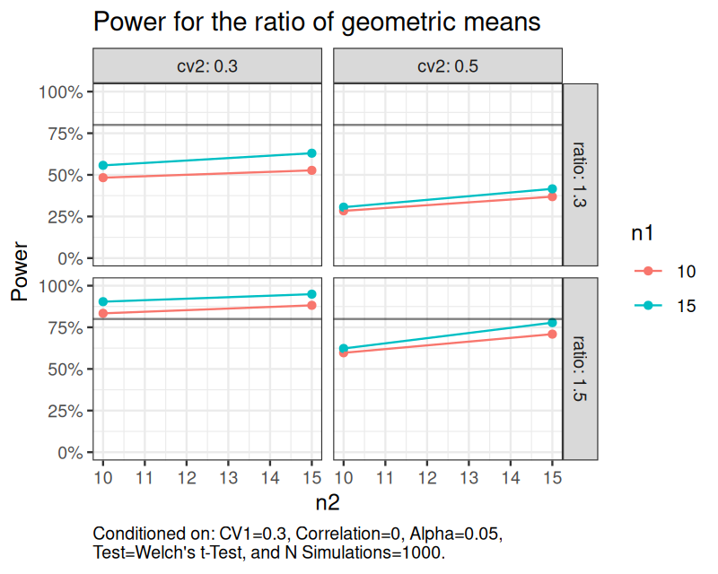
If you are limited by the output from plot.depower(), keep in mind that the
object returned by power() is a standard data frame. This allows
you to easily plot all results with standard plotting functions. In addition,
because plot.depower() uses ggplot2, you can modify the plot as you
normally would. For example:
set.seed(1234)
sim_log_lognormal(
  n1 = c(10, 15),
  n2 = c(10, 15),
  ratio = c(1.3, 1.5),
  cv1 = c(0.3),
  cv2 = c(0.3, 0.5),
  nsims = 1000
) |>
  power(alpha = 0.05) |>
  plot(hline = 0.8, caption_width = 60) +
  ggplot2::theme_bw() +
  ggplot2::theme(plot.caption = ggplot2::element_text(hjust = 0)) +
  ggplot2::labs(title = "Power for the ratio of geometric means")
Value
A ggplot2::ggplot() object.
See Also
Examples
#----------------------------------------------------------------------------
# plot() examples
#----------------------------------------------------------------------------
library(depower)

# Power for independent two-sample t-test
set.seed(1234)
sim_log_lognormal(
  n1 = c(10, 15),
  n2 = c(10, 15),
  ratio = c(1.3, 1.5),
  cv1 = c(0.3),
  cv2 = c(0.3, 0.5),
  nsims = 500
) |>
  power(alpha = 0.05) |>
  plot()

# Power for dependent two-sample t-test
set.seed(1234)
sim_log_lognormal(
  n1 = c(10, 15),
  n2 = c(10, 15),
  ratio = c(1.3, 1.5),
  cv1 = c(0.3, 0.5),
  cv2 = c(0.3, 0.5),
  cor = c(0.3),
  nsims = 500
) |>
  power(alpha = 0.01) |>
  plot()

# Power for two-sample independent AND two-sample dependent t-test
set.seed(1234)
sim_log_lognormal(
  n1 = c(10, 15),
  n2 = c(10, 15),
  ratio = c(1.3, 1.5),
  cv1 = c(0.3),
  cv2 = c(0.3),
  cor = c(0, 0.3, 0.6),
  nsims = 500
) |>
  power(alpha = c(0.05, 0.01)) |>
  plot(facet_row = "cor", color = "test")

# Power for one-sample t-test
set.seed(1234)
sim_log_lognormal(
  n1 = c(10, 15),
  ratio = c(1.2, 1.4),
  cv1 = c(0.3, 0.5),
  nsims = 500
) |>
  power(alpha = c(0.05, 0.01)) |>
  plot()


# Power for independent two-sample NB test
set.seed(1234)
sim_nb(
  n1 = c(10, 15),
  mean1 = 10,
  ratio = c(1.8, 2),
  dispersion1 = 10,
  dispersion2 = 3,
  nsims = 100
) |>
  power(alpha = 0.01) |>
  plot()

# Power for BNB test
set.seed(1234)
sim_bnb(
  n = c(10, 12),
  mean1 = 10,
  ratio = c(1.3, 1.5),
  dispersion = 5,
  nsims = 100
) |>
  power(alpha = 0.01) |>
  plot()
Simulated power
Description
A method to calculate power for objects returned by sim_log_lognormal(),
sim_nb(), and sim_bnb().
Usage
power(data, ..., alpha = 0.05, list_column = FALSE, ncores = 1L)
Arguments
data |
(depower) |
... |
(functions) |
alpha |
(numeric: |
list_column |
(Scalar logical: |
ncores |
(Scalar integer: |
Details
Power is calculated as the proportion of hypothesis tests which result in a
p-value less than or equal to alpha. e.g.
sum(p <= alpha) / nsims
Power is defined as the expected probability of rejecting the null hypothesis for a chosen value of the unknown effect. In a multiple comparisons scenario, power is defined as the marginal power, which is the expected power of the test for each individual null hypothesis assumed to be false.
Other forms of power under the multiple comparisons scenario include
disjunctive or conjunctive power. Disjunctive power is defined as the
expected probability of correctly rejecting one or more null hypotheses.
Conjunctive power is defined as the expected probability of correctly
rejecting all null hypotheses. In the simplest case, and where all hypotheses
are independent, if the marginal power is defined as \pi and m is
the number of null hypotheses assumed to be false, then disjunctive power may
be calculated as 1 - (1 - \pi)^m and conjunctive power may be calculated
as \pi^m. Disjunctive power tends to decrease with increasingly
correlated hypotheses and conjunctive power tends to increase with
increasingly correlated hypotheses.
Argument ...
... are the name-value pairs for the functions used to perform the tests.
If not named, the functions coerced to character will be used for the
name-value pairs. Typical in non-standard evaluation, ... accepts bare
functions and converts them to a list of expressions. Each element in this
list will be validated as a call and then evaluated on the simulated data.
A base::call() is simply an unevaluated function. Below are some examples
of specifying ... in power().
# Examples of specifying ... in power()
data <- sim_nb(
  n1 = 10,
  mean1 = 10,
  ratio = c(1.6, 2),
  dispersion1 = 2,
  dispersion2 = 2,
  nsims = 200
)

# ... is empty, so an appropriate default function will be provided
power(data)

# This is equivalent to leaving ... empty
power(data, "NB Wald test" = wald_test_nb())

# If not named, "wald_test_nb()" will be used to label the function
power(data, wald_test_nb())

# You can specify any parameters in the call. The data argument
# will automatically be inserted or overwritten.
data |>
  power("NB Wald test" = wald_test_nb(equal_dispersion=TRUE, link="log"))

# Multiple functions may be used.
data |>
  power(
    wald_test_nb(link='log'),
    wald_test_nb(link='sqrt'),
    wald_test_nb(link='squared'),
    wald_test_nb(link='identity')
  )

# Just like functions in a pipe, the parentheses are required.
# This will error because wald_test_nb is missing parentheses.
try(power(data, wald_test_nb))
In most cases*, any user created test function may be utilized in ... if the
following conditions are satisfied:
The function contains argument
datawhich is defined as a list with the first and second elements for simulated data.The return object is a list with element
pfor the p-value of the hypothesis test.
Validate with test cases beforehand.
*Simulated data of class log_lognormal_mixed_two_sample has both independent
and dependent data. To ensure the appropriate test function is used,
power.log_lognormal_mixed_two_sample() allows only
t_test_welch() and t_test_paired() in .... Each will
be evaluated on the simulated data according to column data$cor. If one or
both of these functions are not included in ..., the corresponding default
function will be used automatically. If any other test function is included,
an error will be returned.
Argument alpha
\alpha is known as the type I assertion probability and is defined as
the expected probability of rejecting a null hypothesis when it was actually
true. \alpha is compared with the p-value and used as the decision
boundary for rejecting or not rejecting the null hypothesis.
The family-wise error rate is the expected probability of making one or more
type I assertions among a family of hypotheses. Using Bonferroni's method,
\alpha is chosen for the family of hypotheses then divided by the
number of tests performed (m). Each individual hypothesis is tested at
\frac{\alpha}{m}. For example, if you plan to conduct 30 hypothesis
tests and want to control the family-wise error rate to no greater than
\alpha = 0.05, you would set alpha = 0.05/30.
The per-family error rate is the expected number of type I assertions among a
family of hypotheses. If you calculate power for the scenario where you
perform 1,000 hypotheses and want to control the per-family error rate to no
greater than 10 type I assertions, you would choose alpha = 10/1000. This
implicitly assumes all 1,000 hypotheses are truly null. Alternatively, if you
assume 800 of these hypotheses are truly null and 200 are not,
alpha = 10/1000 would control the per-family error rate to no greater than
8 type I assertions. If it is acceptable to keep the per-family error rate as
10, setting alpha = 10/800 would provide greater marginal power than the
previous scenario.
These two methods assume that the distribution of p-values for the truly null hypotheses are uniform(0,1), but remain valid under various other testing scenarios (such as dependent tests). Other multiple comparison methods, such as FDR control, are common in practice but don't directly fit into this power simulation framework.
Column nsims
The final number of valid simulations per unique set of simulation parameters
may be less than the original number requested. This may occur when the test
results in a missing p-value. For wald_test_bnb(), pathological MLE
estimates, generally from small sample sizes and very small dispersions, may
result in a negative estimated standard deviation of the ratio. Thus the test
statistic and p-value would not be calculated. Note that simulated data from
sim_nb() and sim_bnb() may also reduce nsims during the data simulation
phase.
The nsims column in the return data frame is the effective number of
simulations for power results.
Value
A data frame with the following columns appended to the data object:
| Column | Name | Description |
alpha | Type I assertion probability. | |
test | Name-value pair of the function and statistical test: c(as.character(...) = names(...). |
|
data | List-column of simulated data. | |
result | List-column of test results. | |
power | Power of the test for corresponding parameters. |
For power(list_column = FALSE), columns data, and result are excluded from
the data frame.
References
Yu L, Fernandez S, Brock G (2017). “Power analysis for RNA-Seq differential expression studies.” BMC Bioinformatics, 18(1), 234. ISSN 1471-2105, doi:10.1186/s12859-017-1648-2.
Yu L, Fernandez S, Brock G (2020). “Power analysis for RNA-Seq differential expression studies using generalized linear mixed effects models.” BMC Bioinformatics, 21(1), 198. ISSN 1471-2105, doi:10.1186/s12859-020-3541-7.
Rettiganti M, Nagaraja HN (2012). “Power Analyses for Negative Binomial Models with Application to Multiple Sclerosis Clinical Trials.” Journal of Biopharmaceutical Statistics, 22(2), 237–259. ISSN 1054-3406, 1520-5711, doi:10.1080/10543406.2010.528105.
Aban IB, Cutter GR, Mavinga N (2009). “Inferences and power analysis concerning two negative binomial distributions with an application to MRI lesion counts data.” Computational Statistics & Data Analysis, 53(3), 820–833. ISSN 01679473, doi:10.1016/j.csda.2008.07.034.
Julious SA (2004). “Sample sizes for clinical trials with Normal data.” Statistics in Medicine, 23(12), 1921–1986. doi:10.1002/sim.1783.
Vickerstaff V, Omar RZ, Ambler G (2019). “Methods to adjust for multiple comparisons in the analysis and sample size calculation of randomised controlled trials with multiple primary outcomes.” BMC Medical Research Methodology, 19(1), 129. ISSN 1471-2288, doi:10.1186/s12874-019-0754-4.
See Also
Examples
#----------------------------------------------------------------------------
# power() examples
#----------------------------------------------------------------------------
library(depower)

# Power for independent two-sample t-test
set.seed(1234)
data <- sim_log_lognormal(
  n1 = 20,
  n2 = 20,
  ratio = c(1.2, 1.4),
  cv1 = 0.4,
  cv2 = 0.4,
  cor = 0,
  nsims = 1000
)

# Welch's t-test is used by default
power(data)

# But you can specify anything else that is needed
power(
  data = data,
  "Welch's t-Test" = t_test_welch(alternative = "greater"),
  alpha = 0.01
)

# Power for dependent two-sample t-test
set.seed(1234)
sim_log_lognormal(
  n1 = 20,
  n2 = 20,
  ratio = c(1.2, 1.4),
  cv1 = 0.4,
  cv2 = 0.4,
  cor = 0.5,
  nsims = 1000
) |>
  power()

# Power for mixed-type two-sample t-test
set.seed(1234)
sim_log_lognormal(
  n1 = 20,
  n2 = 20,
  ratio = c(1.2, 1.4),
  cv1 = 0.4,
  cv2 = 0.4,
  cor = c(0, 0.5),
  nsims = 1000
) |>
  power()

# Power for one-sample t-test
set.seed(1234)
sim_log_lognormal(
  n1 = 20,
  ratio = c(1.2, 1.4),
  cv1 = 0.4,
  nsims = 1000
) |>
  power()

# Power for independent two-sample NB test
set.seed(1234)
sim_nb(
  n1 = 10,
  mean1 = 10,
  ratio = c(1.6, 2),
  dispersion1 = 2,
  dispersion2 = 2,
  nsims = 200
) |>
  power()

# Power for BNB test
set.seed(1234)
sim_bnb(
  n = 10,
  mean1 = 10,
  ratio = c(1.4, 1.6),
  dispersion = 10,
  nsims = 200
) |>
  power()
Simulate data from a BNB distribution
Description
Simulate data from the bivariate negative binomial (BNB) distribution. The
BNB distribution is used to simulate count data where the event counts are
jointly dependent (correlated). For independent data, see
sim_nb().
Usage
sim_bnb(
  n,
  mean1,
  mean2,
  ratio,
  dispersion,
  nsims = 1L,
  return_type = "list",
  max_zeros = 0.99
)
Arguments
n |
(integer: |
mean1 |
(numeric: |
mean2, ratio |
(numeric:
|
dispersion |
(numeric: |
nsims |
(Scalar integer: |
return_type |
(string: |
max_zeros |
(Scalar numeric: |
Details
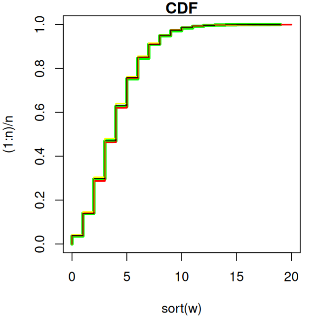
The negative binomial distribution may be defined using a gamma-Poisson
mixture distribution. In this case, the Poisson parameter \lambda
is a random variable with gamma distribution. Equivalence between different
parameterizations are demonstrated below:
# Define constants and their relationships
n <- 10000
dispersion <- 8
mu <- 4
p <- dispersion / (dispersion + mu)
q <- mu / (mu + dispersion)
variance <- mu + (mu^2 / dispersion)
rate <- p / (1 - p)
scale <- (1 - p) / p

# alternative formula for mu
mu_alt <- (dispersion * (1 - p)) / p
stopifnot(isTRUE(all.equal(mu, mu_alt)))

set.seed(20240321)

# Using built-in rnbinom with dispersion and mean
w <- rnbinom(n = n, size = dispersion, mu = mu)

# Using gamma-Poisson mixture with gamma rate parameter
x <- rpois(
  n = n,
  lambda = rgamma(n = n, shape = dispersion, rate = rate)
)

# Using gamma-Poisson mixture with gamma scale parameter
y <- rpois(
  n = n,
  lambda = rgamma(n = n, shape = dispersion, scale = scale)
)

# Using gamma-Poisson mixture with multiplicative mean and
# gamma scale parameter
z <- rpois(
  n = n,
  lambda = mu * rgamma(n = n, shape = dispersion, scale = 1/dispersion)
)

# Compare CDFs
par(mar=c(4,4,1,1))
plot(
  x = sort(w),
  y = (1:n)/n,
  xlim = range(c(w,x,y,z)),
  ylim = c(0,1),
  col = 'green',
  lwd = 4,
  type = 'l',
  main = 'CDF'
)
lines(x = sort(x), y = (1:n)/n, col = 'red', lwd = 2)
lines(x = sort(y), y = (1:n)/n, col = 'yellow', lwd = 1.5)
lines(x = sort(z), y = (1:n)/n, col = 'black')
The BNB distribution is implemented by compounding two conditionally
independent Poisson random variables X_1 \mid G = g \sim \text{Poisson}(\mu g)
and X_2 \mid G = g \sim \text{Poisson}(r \mu g) with a gamma random
variable G \sim \text{Gamma}(\theta, \theta^{-1}). The probability mass
function for the joint distribution of X_1, X_2 is
P(X_1 = x_1, X_2 = x_2) = \frac{\Gamma(x_1 + x_2 + \theta)}{(\mu + r \mu + \theta)^{x_1 + x_2 + \theta}}
  \frac{\mu^{x_1}}{x_1!} \frac{(r \mu)^{x_2}}{x_2!}
  \frac{\theta^{\theta}}{\Gamma(\theta)}
where x_1,x_2 \in \mathbb{N}^{\geq 0} are specific values of the count
outcomes, \theta \in \mathbb{R}^{> 0} is the dispersion parameter
which controls the dispersion and level of correlation between the two
samples (otherwise known as the shape parameter of the gamma distribution),
\mu \in \mathbb{R}^{> 0} is the mean parameter, and
r = \frac{\mu_2}{\mu_1} \in \mathbb{R}^{> 0} is the ratio parameter
representing the multiplicative change in the mean of the second sample
relative to the first sample. G denotes the random subject effect and
the gamma distribution scale parameter is assumed to be the inverse of the
dispersion parameter (\theta^{-1}) for identifiability.
Correlation decreases from 1 to 0 as the dispersion parameter increases from 0 to infinity. For a given dispersion, increasing means also increases the correlation. See 'Examples' for a demonstration.
See 'Details' in sim_nb() for additional information on the
negative binomial distribution.
Value
If nsims = 1 and the number of unique parameter combinations is
one, the following objects are returned:
If
return_type = "list", a list:Slot Name Description 1 Simulated counts from sample 1. 2 Simulated counts from sample 2. If
return_type = "data.frame", a data frame:Column Name Description 1 itemSubject/item indicator. 2 conditionSample/condition indicator. 3 valueSimulated counts.
If nsims > 1 or the number of unique parameter combinations is greater than
one, each object described above is returned in a list-column named data in
a depower simulation data frame:
| Column | Name | Description |
| 1 | n1 | Sample size of sample 1. |
| 2 | n2 | Sample size of sample 2. |
| 3 | mean1 | Mean for sample 1. |
| 4 | mean2 | Mean for sample 2. |
| 5 | ratio | Ratio of means (sample 2 / sample 1). |
| 6 | dispersion | Gamma distribution shape parameter (dispersion). |
| 7 | nsims | Number of valid simulation iterations. |
| 8 | distribution | Distribution sampled from. |
| 9 | data | List-column of simulated data. |
References
Yu L, Fernandez S, Brock G (2020). “Power analysis for RNA-Seq differential expression studies using generalized linear mixed effects models.” BMC Bioinformatics, 21(1), 198. ISSN 1471-2105, doi:10.1186/s12859-020-3541-7.
Rettiganti M, Nagaraja HN (2012). “Power Analyses for Negative Binomial Models with Application to Multiple Sclerosis Clinical Trials.” Journal of Biopharmaceutical Statistics, 22(2), 237–259. ISSN 1054-3406, 1520-5711, doi:10.1080/10543406.2010.528105.
Aban IB, Cutter GR, Mavinga N (2009). “Inferences and power analysis concerning two negative binomial distributions with an application to MRI lesion counts data.” Computational Statistics & Data Analysis, 53(3), 820–833. ISSN 01679473, doi:10.1016/j.csda.2008.07.034.
See Also
Examples
#----------------------------------------------------------------------------
# sim_bnb() examples
#----------------------------------------------------------------------------
library(depower)

# Paired two-sample data returned in a data frame
sim_bnb(
  n = 10,
  mean1 = 10,
  ratio = 1.6,
  dispersion = 3,
  nsims = 1,
  return_type = "data.frame"
)

# Paired two-sample data returned in a list
sim_bnb(
  n = 10,
  mean1 = 10,
  ratio = 1.6,
  dispersion = 3,
  nsims = 1,
  return_type = "list"
)

# Two simulations of paired two-sample data
# returned as a list of data frames
sim_bnb(
  n = 10,
  mean1 = 10,
  ratio = 1.6,
  dispersion = 3,
  nsims = 2,
  return_type = "data.frame"
)

# Two simulations of Paired two-sample data
# returned as a list of lists
sim_bnb(
  n = 10,
  mean1 = 10,
  ratio = 1.6,
  dispersion = 3,
  nsims = 2,
  return_type = "list"
)

#----------------------------------------------------------------------------
# Visualization of the BNB distribution as dispersion varies.
#----------------------------------------------------------------------------
set.seed(1234)
data <- lapply(
  X = c(1, 10, 100, 1000),
  FUN = function(x) {
    d <- sim_bnb(
      n = 1000,
      mean1 = 10,
      ratio = 1.5,
      dispersion = x,
      nsims = 1,
      return_type = "data.frame"
    )
    cor <- cor(
      x = d[d$condition == "1", ]$value,
      y = d[d$condition == "2", ]$value
    )
    cbind(dispersion = x, correlation = cor, d)
  }
)

data <- do.call(what = "rbind", args = data)

ggplot2::ggplot(
  data = data,
  mapping = ggplot2::aes(x = value, fill = condition)
) +
  ggplot2::facet_wrap(
    facets = ggplot2::vars(.data$dispersion),
    ncol = 2,
    labeller = ggplot2::labeller(.rows = ggplot2::label_both)
  ) +
  ggplot2::geom_density(alpha = 0.3) +
  ggplot2::coord_cartesian(xlim = c(0, 60)) +
  ggplot2::geom_text(
    mapping = ggplot2::aes(
      x = 30,
      y = 0.12,
      label = paste0("Correlation: ", round(correlation, 2))
    ),
    check_overlap = TRUE
  ) +
  ggplot2::labs(
    x = "Value",
    y = "Density",
    fill = "Condition",
    caption = "Mean1=10, Mean2=15, ratio=1.5"
  )
Simulate data from a normal distribution
Description
Simulate data from the log transformed lognormal distribution (i.e. a normal distribution). This function handles all three cases:
One-sample data
Dependent two-sample data
Independent two-sample data
Usage
sim_log_lognormal(
  n1,
  n2 = NULL,
  ratio,
  cv1,
  cv2 = NULL,
  cor = 0,
  nsims = 1L,
  return_type = "list",
  messages = TRUE
)
Arguments
n1 |
(integer: |
n2 |
(integer: |
ratio |
(numeric:
See 'Details' for additional information. |
cv1 |
(numeric: |
cv2 |
(numeric: |
cor |
(numeric: |
nsims |
(Scalar integer: |
return_type |
(string: |
messages |
(Scalar logical: |
Details
Based on assumed characteristics of the original lognormal distribution, data is simulated from the corresponding log-transformed (normal) distribution. This simulated data is suitable for assessing power of a hypothesis for the geometric mean or ratio of geometric means from the original lognormal data.
This method can also be useful for other population distributions which are positive and where it makes sense to describe the ratio of geometric means. However, the lognormal distribution is theoretically correct in the sense that you can log transform to a normal distribution, compute the summary statistic, then apply the inverse transformation to summarize on the original lognormal scale.
Let GM(\cdot) be the geometric mean and AM(\cdot) be the
arithmetic mean. For independent lognormal samples X_1 and X_2
\text{Fold Change} = \frac{GM(X_2)}{GM(X_1)}
For dependent lognormal samples X_1 and X_2
\text{Fold Change} = GM\left( \frac{X_2}{X_1} \right)
Unlike ratios and the arithmetic mean, for equal sample sizes of
X_1 and X_2 it follows that
\frac{GM(X_2)}{GM(X_1)} = GM \left( \frac{X_2}{X_1} \right) =
e^{AM(\ln X_2) - AM(\ln X_1)} = e^{AM(\ln X_2 - \ln X_1)}
.
The coefficient of variation (CV) for X is defined as
CV = \frac{SD(X)}{AM(X)}
The relationship between sample statistics for the original lognormal data
(X) and the natural logged data (\ln{X}) are
\begin{aligned}
AM(X)  &= e^{AM(\ln{X}) + \frac{Var(\ln{X})}{2}} \\
GM(X)  &= e^{AM(\ln{X})} \\
Var(X) &= AM(X)^2 \left( e^{Var(\ln{X})} - 1 \right) \\
CV(X)  &= \frac{\sqrt{AM(X)^2 \left( e^{Var(\ln{X})} - 1 \right)}}{AM(X)} \\
       &= \sqrt{e^{Var(\ln{X})} - 1}
\end{aligned}
and
\begin{aligned}
AM(\ln{X})  &= \ln \left( \frac{AM(X)}{\sqrt{CV(X)^2 + 1}} \right) \\
Var(\ln{X}) &= \ln(CV(X)^2 + 1) \\
Cor(\ln{X_1}, \ln{X_2}) &= \frac{\ln \left( Cor(X_1, X_2)CV(X_1)CV(X_2) + 1 \right)}{SD(\ln{X_1})SD(\ln{X_2})}
\end{aligned}
Based on the properties of correlation and variance,
\begin{aligned}
Var(X_2 - X_1) &= Var(X_1) + Var(X_2) - 2Cov(X_1, X_2) \\
           &= Var(X_1) + Var(X_2) - 2Cor(X_1, X_2)SD(X_1)SD(X_2) \\
SD(X_2 - X_1)  &= \sqrt{Var(X_2 - X_1)}
\end{aligned}
The standard deviation of the differences gets smaller the more positive the correlation and conversely gets larger the more negative the correlation. For the special case where the two samples are uncorrelated and each has the same variance, it follows that
\begin{aligned}
Var(X_2 - X_1) &= \sigma^2 + \sigma^2 \\
SD(X_2 - X_1) &= \sqrt{2}\sigma
\end{aligned}
Value
If nsims = 1 and the number of unique parameter combinations is
one, the following objects are returned:
If one-sample data with
return_type = "list", a list:Slot Name Description 1 One sample of simulated normal values. If one-sample data with
return_type = "data.frame", a data frame:Column Name Description 1 itemPair/subject/item indicator. 2 valueSimulated normal values. If two-sample data with
return_type = "list", a list:Slot Name Description 1 Simulated normal values from sample 1. 2 Simulated normal values from sample 2. If two-sample data with
return_type = "data.frame", a data frame:Column Name Description 1 itemPair/subject/item indicator. 2 conditionTime/group/condition indicator. 3 valueSimulated normal values.
If nsims > 1 or the number of unique parameter combinations is greater than
one, each object described above is returned in data frame, located in a
list-column named data.
If one-sample data, a data frame:
Column Name Description 1 n1The sample size. 2 ratioGeometric mean [GM(sample 1)]. 3 cv1Coefficient of variation for sample 1. 4 nsimsNumber of data simulations. 5 distributionDistribution sampled from. 6 dataList-column of simulated data. If two-sample data, a data frame:
Column Name Description 1 n1Sample size of sample 1. 2 n2Sample size of sample 2. 3 ratioRatio of geometric means [GM(sample 2) / GM(sample 1)] or geometric mean ratio [GM(sample 2 / sample 1)]. 4 cv1Coefficient of variation for sample 1. 5 cv2Coefficient of variation for sample 2. 6 corCorrelation between samples. 7 nsimsNumber of data simulations. 8 distributionDistribution sampled from. 9 dataList-column of simulated data.
References
Julious SA (2004). “Sample sizes for clinical trials with Normal data.” Statistics in Medicine, 23(12), 1921–1986. doi:10.1002/sim.1783.
Hauschke D, Steinijans VW, Diletti E, Burke M (1992). “Sample size determination for bioequivalence assessment using a multiplicative model.” Journal of Pharmacokinetics and Biopharmaceutics, 20(5), 557–561. ISSN 0090-466X, doi:10.1007/BF01061471.
Johnson NL, Kotz S, Balakrishnan N (1994). Continuous univariate distributions, Wiley series in probability and mathematical statistics, 2nd ed edition. Wiley, New York. ISBN 9780471584957 9780471584940.
Examples
#----------------------------------------------------------------------------
# sim_log_lognormal() examples
#----------------------------------------------------------------------------
library(depower)

# Independent two-sample data returned in a data frame
sim_log_lognormal(
  n1 = 10,
  n2 = 10,
  ratio = 1.3,
  cv1 = 0.35,
  cv2 = 0.35,
  cor = 0,
  nsims = 1,
  return_type = "data.frame"
)

# Independent two-sample data returned in a list
sim_log_lognormal(
  n1 = 10,
  n2 = 10,
  ratio = 1.3,
  cv1 = 0.35,
  cv2 = 0.35,
  cor = 0,
  nsims = 1,
  return_type = "list"
)

# Dependent two-sample data returned in a data frame
sim_log_lognormal(
  n1 = 10,
  n2 = 10,
  ratio = 1.3,
  cv1 = 0.35,
  cv2 = 0.35,
  cor = 0.4,
  nsims = 1,
  return_type = "data.frame"
)

# Dependent two-sample data returned in a list
sim_log_lognormal(
  n1 = 10,
  n2 = 10,
  ratio = 1.3,
  cv1 = 0.35,
  cv2 = 0.35,
  cor = 0.4,
  nsims = 1,
  return_type = "list"
)

# One-sample data returned in a data frame
sim_log_lognormal(
  n1 = 10,
  ratio = 1.3,
  cv1 = 0.35,
  nsims = 1,
  return_type = "data.frame"
)

# One-sample data returned in a list
sim_log_lognormal(
  n1 = 10,
  ratio = 1.3,
  cv1 = 0.35,
  nsims = 1,
  return_type = "list"
)

# Independent two-sample data: two simulations for four parameter combinations.
# Returned as a list-column of lists within a data frame
sim_log_lognormal(
  n1 = c(10, 20),
  n2 = c(10, 20),
  ratio = 1.3,
  cv1 = 0.35,
  cv2 = 0.35,
  cor = 0,
  nsims = 2,
  return_type = "list"
)

# Dependent two-sample data: two simulations for two parameter combinations.
# Returned as a list-column of lists within a data frame
sim_log_lognormal(
  n1 = c(10, 20),
  n2 = c(10, 20),
  ratio = 1.3,
  cv1 = 0.35,
  cv2 = 0.35,
  cor = 0.4,
  nsims = 2,
  return_type = "list"
)

# One-sample data: two simulations for two parameter combinations
# Returned as a list-column of lists within a data frame
sim_log_lognormal(
  n1 = c(10, 20),
  ratio = 1.3,
  cv1 = 0.35,
  nsims = 2,
  return_type = "list"
)
Simulate data from a NB distribution
Description
Simulate data from two independent negative binomial (NB) distributions. For
paired data, see sim_bnb().
Usage
sim_nb(
  n1,
  n2 = n1,
  mean1,
  mean2,
  ratio,
  dispersion1,
  dispersion2 = dispersion1,
  nsims = 1L,
  return_type = "list",
  max_zeros = 0.99
)
Arguments
n1 |
(integer: |
n2 |
(integer: |
mean1 |
(numeric: |
mean2, ratio |
(numeric:
|
dispersion1 |
(numeric: |
dispersion2 |
(numeric: |
nsims |
(Scalar integer: |
return_type |
(string: |
max_zeros |
(Scalar numeric: |
Details
The negative binomial distribution has many parameterizations. In the regression modeling context, it is common to specify the distribution in terms of its mean and dispersion. We use the following probability mass function:
\begin{aligned}
P(X = x) &= \dbinom{x + \theta - 1}{x}
            \left( \frac{\theta}{\theta + \mu} \right)^{\theta}
            \left( \frac{\mu}{\mu + \theta} \right)^x \\
         &= \frac{\Gamma(x + \theta)}{x! \Gamma(\theta)}
            \left( \frac{\theta}{\theta + \mu} \right)^{\theta}
            \left( \frac{\mu}{\mu + \theta} \right)^{x} \\
         &= \frac{\Gamma(x + \theta)}{(\theta + \mu)^{\theta + x}}
            \frac{\theta^{\theta}}{\Gamma(\theta)} \frac{\mu^{x}}{x!}
\end{aligned}
where x \in \mathbb{N}^{\geq 0}, \theta \in \mathbb{R}^{> 0}
is the dispersion parameter, and \mu \in \mathbb{R}^{> 0} is the mean.
This is analogous to the typical formulation where X is counting
x failures given \theta successes and
p = \frac{\theta}{\theta + \mu} is the probability of success on each
trial. It follows that E(X) = \mu and
Var(X) = \mu + \frac{\mu^2}{\theta}. The \theta parameter
describes the 'dispersion' among observations. Smaller values of \theta
lead to overdispersion and larger values of \theta decrease the
overdispersion, eventually converging to the Poisson distribution.
Described above is the 'indirect quadratic parameterization' of the negative
binomial distribution, which is commonly found in the R ecosystem. However, it
is somewhat counterintuitive because the smaller \theta gets, the larger
the overdispersion. The 'direct quadratic parameterization' of the negative
binomial distribution may be found in some R packages and other languages
such as SAS and Stata. The direct parameterization is defined by substituting
\alpha = \frac{1}{\theta} (\alpha > 0) which results in
Var(X) = \mu + \alpha\mu^2. In this case, the larger \alpha gets
the larger the overdispersion, and the Poisson distribution is a special case
of the negative binomial distribution where \alpha = 0.
A general class of negative binomial models may be defined with mean
\mu and variance \mu + \alpha\mu^{p}. The 'linear
parameterization' is then found by setting p=1, resulting in
Var(X) = \mu + \alpha\mu. It's common to label the linear
parameterization as 'NB1' and the direct quadratic parameterization as 'NB2'.
See 'Details' in sim_bnb() for additional information on the
gamma-Poisson mixture formulation of the negative binomial distribution.
Value
If nsims = 1 and the number of unique parameter combinations is
one, the following objects are returned:
If
return_type = "list", a list:Slot Name Description 1 value1Simulated counts from group 1. 2 value2Simulated counts from group 2. If
return_type = "data.frame", a data frame:Column Name Description 1 itemSubject/item indicator. 2 conditionGroup/condition indicator. 3 valueSimulated counts.
If nsims > 1 or the number of unique parameter combinations is greater than
one, each object described above is returned in a list-column named data in
a depower simulation data frame:
| Column | Name | Description |
| 1 | n1 | Sample size of group 1. |
| 2 | n2 | Sample size of group 2. |
| 3 | mean1 | Mean for group 1. |
| 4 | mean2 | Mean for group 2. |
| 5 | ratio | Ratio of means (group 2 / group 1). |
| 6 | dispersion1 | Dispersion parameter for group 1. |
| 7 | dispersion2 | Dispersion parameter for group 2. |
| 8 | nsims | Number of valid simulation iterations. |
| 9 | distribution | Distribution sampled from. |
| 10 | data | List-column of simulated data. |
References
Yu L, Fernandez S, Brock G (2017). “Power analysis for RNA-Seq differential expression studies.” BMC Bioinformatics, 18(1), 234. ISSN 1471-2105, doi:10.1186/s12859-017-1648-2.
Rettiganti M, Nagaraja HN (2012). “Power Analyses for Negative Binomial Models with Application to Multiple Sclerosis Clinical Trials.” Journal of Biopharmaceutical Statistics, 22(2), 237–259. ISSN 1054-3406, 1520-5711, doi:10.1080/10543406.2010.528105.
Aban IB, Cutter GR, Mavinga N (2009). “Inferences and power analysis concerning two negative binomial distributions with an application to MRI lesion counts data.” Computational Statistics & Data Analysis, 53(3), 820–833. ISSN 01679473, doi:10.1016/j.csda.2008.07.034.
Hilbe JM (2011). Negative Binomial Regression, 2 edition. Cambridge University Press. ISBN 9780521198158 9780511973420, doi:10.1017/CBO9780511973420.
Hilbe JM (2014). Modeling count data. Cambridge University Press, New York, NY. ISBN 9781107028333 9781107611252, doi:10.1017/CBO9781139236065.
Cameron AC, Trivedi PK (2013). Regression Analysis of Count Data, Econometric Society Monographs, 2 edition. Cambridge University Press. doi:10.1017/CBO9781139013567.
See Also
Examples
#----------------------------------------------------------------------------
# sim_nb() examples
#----------------------------------------------------------------------------
library(depower)

# Independent two-sample NB data returned in a data frame
sim_nb(
  n1 = 10,
  mean1 = 5,
  ratio = 1.6,
  dispersion1 = 0.5,
  dispersion2 = 0.5,
  nsims = 1,
  return_type = "data.frame"
)

# Independent two-sample NB data returned in a list
sim_nb(
  n1 = 10,
  mean1 = 5,
  ratio = 1.6,
  dispersion1 = 0.5,
  dispersion2 = 0.5,
  nsims = 1,
  return_type = "list"
)

# Two simulations of independent two-sample data
# returned as a list of data frames
sim_nb(
  n1 = 10,
  mean1 = 5,
  ratio = 1.6,
  dispersion1 = 0.5,
  dispersion2 = 0.5,
  nsims = 2,
  return_type = "data.frame"
)

# Two simulations of independent two-sample data
# returned as a list of lists
sim_nb(
  n1 = 10,
  mean1 = 5,
  ratio = 1.6,
  dispersion1 = 0.5,
  dispersion2 = 0.5,
  nsims = 2,
  return_type = "list"
)

#----------------------------------------------------------------------------
# Visualization of the NB distribution as dispersion varies between groups.
#----------------------------------------------------------------------------
disp <- expand.grid(c(1, 10, 100), c(1, 10, 100))
set.seed(1234)
data <- mapply(
  FUN = function(disp1, disp2) {
    d <- sim_nb(
      n1 = 1000,
      mean1 = 10,
      ratio = 1.5,
      dispersion1 = disp1,
      dispersion2 = disp2,
      nsims = 1,
      return_type = "data.frame"
    )
    cbind(dispersion1 = disp1, dispersion2 = disp2, d)
  },
  disp1 = disp[[1]],
  disp2 = disp[[2]],
  SIMPLIFY = FALSE
)

data <- do.call(what = "rbind", args = data)

ggplot2::ggplot(
  data = data,
  mapping = ggplot2::aes(x = value, fill = condition)
) +
  ggplot2::facet_grid(
    rows = ggplot2::vars(.data$dispersion2),
    cols = ggplot2::vars(.data$dispersion1),
    labeller = ggplot2::labeller(
      .rows = ggplot2::label_both,
      .cols = ggplot2::label_both
    )
  ) +
  ggplot2::geom_density(alpha = 0.3) +
  ggplot2::coord_cartesian(xlim = c(0, 50)) +
  ggplot2::labs(
    x = "Value",
    y = "Density",
    fill = "Condition",
    caption = "Mean1=10, Mean2=15, ratio=1.5"
  )
Paired and one-sample t-Tests
Description
Performs paired and one-sample t-Tests.
Usage
t_test_paired(data, alternative = "two.sided", ci_level = NULL, mean_null = 0)
Arguments
data |
(list) |
alternative |
(string: |
ci_level |
(Scalar numeric: |
mean_null |
(Scalar numeric: |
Details
This function is primarily designed for speed in simulation. Missing values are silently excluded.
The one-sample test is used for both the true one-sample scenario and for the paired differences from a dependent two-sample scenario. Below we use paired difference language as that is the most common case. The hypotheses for the paired t-test are
\begin{aligned}
H_{null} &: \mu_{diff} = \mu_{null} \\
H_{alt} &: \begin{cases}
  \mu_{diff} \neq \mu_{null} & \text{two-sided}\\
  \mu_{diff} > \mu_{null} & \text{greater than}\\
  \mu_{diff} < \mu_{null} & \text{less than}
\end{cases}
\end{aligned}
where \mu_{diff} = AM(X_2 - X_1) is the arithmetic mean of the paired
differences (sample 2 - sample 1) and \mu_{null} is a constant for the
assumed population mean difference (usually \mu_{null} = 0).
The test statistic is
T = \frac{\bar{x}_{diff} - \mu_{null}}{\sqrt{\frac{s^2}{n}}}
where \bar{x}_{diff} is the sample mean of the differences, \mu_{null}
is the population mean difference assumed under the null hypothesis, n
is the sample size of the differences, and s^2 is the sample variance.
The critical value of the test statistic has degrees of freedom
df = n-1
and the p-value is calculated as
\begin{aligned}
p &= \begin{cases}
  2 \text{min} \{P(T \geq t_{n-1} \mid H_{null}), P(T \leq t_{n-1} \mid H_{null})\} & \text{two-sided}\\
  P(T \geq t_{n-1} \mid H_{null}) & \text{greater than}\\
  P(T \leq t_{n-1} \mid H_{null}) & \text{less than}
\end{cases}
\end{aligned}
Let GM(\cdot) be the geometric mean and AM(\cdot) be the
arithmetic mean. For dependent lognormal samples X_1 and X_2 it
follows that \ln X_1 and \ln X_2 are dependent normally
distributed variables. Setting \mu_{diff} = AM(\ln X_2 - \ln X_1)
we have
e^{\mu_{diff}} = GM\left( \frac{X_2}{X_1} \right)
This forms the basis for making inference about the geometric mean ratio of the original lognormal data using the mean difference of the log transformed normal data.
Value
A list with the following elements:
| Slot | Subslot | Name | Description |
| 1 | t | Value of the t-statistic. | |
| 2 | df | Degrees of freedom for the t-statistic. | |
| 3 | p | p-value. | |
| 4 | mean_diff | Estimated mean or mean of the differences (sample 2 – sample 1). | |
| 4 | 1 | estimate | Point estimate. |
| 4 | 2 | lower | Confidence interval lower bound. |
| 4 | 3 | upper | Confidence interval upper bound. |
| 5 | n | Number of paired observations. | |
| 6 | method | Method used for the results. | |
| 7 | alternative | The alternative hypothesis. | |
| 8 | ci_level | The confidence level. | |
| 9 | mean_null | Assumed population mean of the differences under the null hypothesis. |
References
Julious SA (2004). “Sample sizes for clinical trials with Normal data.” Statistics in Medicine, 23(12), 1921–1986. doi:10.1002/sim.1783.
Hauschke D, Steinijans VW, Diletti E, Burke M (1992). “Sample size determination for bioequivalence assessment using a multiplicative model.” Journal of Pharmacokinetics and Biopharmaceutics, 20(5), 557–561. ISSN 0090-466X, doi:10.1007/BF01061471.
Johnson NL, Kotz S, Balakrishnan N (1994). Continuous univariate distributions, Wiley series in probability and mathematical statistics, 2nd ed edition. Wiley, New York. ISBN 9780471584957 9780471584940.
See Also
Examples
#----------------------------------------------------------------------------
# t_test_paired() examples
#----------------------------------------------------------------------------
library(depower)

# One-sample t-test
set.seed(1234)
t_test1 <- sim_log_lognormal(
  n1 = 40,
  ratio = 1.5,
  cv1 = 0.4
) |>
  t_test_paired(ci_level = 0.95)

t_test1

# Paired t-test using two dependent samples
set.seed(1234)
t_test2 <- sim_log_lognormal(
  n1 = 40,
  n2 = 40,
  ratio = 1.5,
  cv1 = 0.4,
  cv2 = 0.2,
  cor = 0.3
) |>
  t_test_paired(ci_level = 0.95)

t_test2
Welch's t-Test
Description
Performs Welch's independent two-sample t-test.
Usage
t_test_welch(data, alternative = "two.sided", ci_level = NULL, mean_null = 0)
Arguments
data |
(list) |
alternative |
(string: |
ci_level |
(Scalar numeric: |
mean_null |
(Scalar numeric: |
Details
This function is primarily designed for speed in simulation. Missing values are silently excluded.
The hypotheses for Welch's independent two-sample t-test are
\begin{aligned}
H_{null} &: \mu_2 - \mu_1 = \mu_{null} \\
H_{alt} &: \begin{cases}
  \mu_2 - \mu_1 \neq \mu_{null} & \text{two-sided}\\
  \mu_2 - \mu_1 > \mu_{null} & \text{greater than}\\
  \mu_2 - \mu_1 < \mu_{null} & \text{less than}
\end{cases}
\end{aligned}
where \mu_1 is the population mean of group 1, \mu_2 is the
population mean of group 2, and \mu_{null} is a constant for the assumed
difference of population means (usually \mu_{null} = 0).
The test statistic is
T = \frac{(\bar{x}_2 - \bar{x}_1) - \mu_{null}}{\sqrt{\frac{s_1^2}{n_1} + \frac{s_2^2}{n_2}}}
where \bar{x}_1 and \bar{x}_2 are the sample means, \mu_{null}
is the difference of population means assumed under the null hypothesis,
n_1 and n_2 are the sample sizes, and s_1^2 and s_2^2
are the sample variances.
The critical value of the test statistic uses the Welch–Satterthwaite degrees of freedom
v = \frac{\left( \frac{s_1^2}{n_1} + \frac{s_2^2}{n_2} \right)^2}
         {(N_1 - 1)^{-1}\left( \frac{s_1^2}{n_1} \right)^2 +
         (N_2 - 1)^{-1}\left( \frac{s_2^2}{n_2} \right)^2}
and the p-value is calculated as
\begin{aligned}
p &= \begin{cases}
  2 \text{min} \{P(T \geq t_{v} \mid H_{null}), P(T \leq t_{v} \mid H_{null})\} & \text{two-sided}\\
  P(T \geq t_{v} \mid H_{null}) & \text{greater than}\\
  P(T \leq t_{v} \mid H_{null}) & \text{less than}
\end{cases}
\end{aligned}
Let GM(\cdot) be the geometric mean and AM(\cdot) be the
arithmetic mean. For independent lognormal variables X_1 and X_2
it follows that \ln X_1 and \ln X_2 are independent normally
distributed variables. Defining
\mu_{X_2} - \mu_{X_1} = AM(\ln X_2) - AM(\ln X_1)
we have
e^{\mu_{X_2} - \mu_{X_1}} = \frac{GM(X_2)}{GM(X_1)}
This forms the basis for making inference about the ratio of geometric means of the original lognormal data using the difference of means of the log transformed normal data.
Value
A list with the following elements:
| Slot | Subslot | Name | Description |
| 1 | t | Value of the t-statistic. | |
| 2 | df | Degrees of freedom for the t-statistic. | |
| 3 | p | p-value. | |
| 4 | diff_mean | Estimated difference of means (group 2 – group 1). | |
| 4 | 1 | estimate | Point estimate. |
| 4 | 2 | lower | Confidence interval lower bound. |
| 4 | 3 | upper | Confidence interval upper bound. |
| 5 | mean1 | Estimated mean of group 1. | |
| 6 | mean2 | Estimated mean of group 2. | |
| 7 | n1 | Sample size of group 1. | |
| 8 | n2 | Sample size of group 2. | |
| 9 | method | Method used for the results. | |
| 10 | alternative | The alternative hypothesis. | |
| 11 | ci_level | The confidence level. | |
| 12 | mean_null | Assumed population difference of the means under the null hypothesis. |
References
Julious SA (2004). “Sample sizes for clinical trials with Normal data.” Statistics in Medicine, 23(12), 1921–1986. doi:10.1002/sim.1783.
Hauschke D, Steinijans VW, Diletti E, Burke M (1992). “Sample size determination for bioequivalence assessment using a multiplicative model.” Journal of Pharmacokinetics and Biopharmaceutics, 20(5), 557–561. ISSN 0090-466X, doi:10.1007/BF01061471.
Johnson NL, Kotz S, Balakrishnan N (1994). Continuous univariate distributions, Wiley series in probability and mathematical statistics, 2nd ed edition. Wiley, New York. ISBN 9780471584957 9780471584940.
See Also
Examples
#----------------------------------------------------------------------------
# t_test_welch() examples
#----------------------------------------------------------------------------
library(depower)

# Welch's t-test
set.seed(1234)
sim_log_lognormal(
  n1 = 40,
  n2 = 40,
  ratio = 1.5,
  cv1 = 0.4,
  cv2 = 0.4
) |>
  t_test_welch(ci_level = 0.95)
Wald test for BNB ratio of means
Description
Wald test for the ratio of means from bivariate negative binomial outcomes.
Usage
wald_test_bnb(
  data,
  ci_level = NULL,
  link = "log",
  ratio_null = 1,
  distribution = asymptotic(),
  ...
)
Arguments
data |
(list) |
ci_level |
(Scalar numeric: |
link |
(Scalar string: |
ratio_null |
(Scalar numeric: |
distribution |
(function: |
... |
Optional arguments passed to the MLE function |
Details
This function is primarily designed for speed in simulation. Missing values are silently excluded.
Suppose X_1 \mid G = g \sim \text{Poisson}(\mu g) and
X_2 \mid G = g \sim \text{Poisson}(r \mu g) where
G \sim \text{Gamma}(\theta, \theta^{-1}) is the random item (subject)
effect. Then X_1, X_2 \sim \text{BNB}(\mu, r, \theta) is the joint
distribution where X_1 and X_2 are dependent (though conditionally
independent), X_1 is the count outcome for sample 1 of the items
(subjects), X_2 is the count outcome for sample 2 of the items (subjects),
\mu is the conditional mean of sample 1, r is the ratio of the
conditional means of sample 2 with respect to sample 1, and \theta is
the gamma distribution shape parameter which controls the dispersion and the
correlation between sample 1 and 2.
The hypotheses for the Wald test of r are
\begin{aligned}
H_{null} &: f(r) = f(r_{null}) \\
H_{alt} &: f(r) \neq f(r_{null})
\end{aligned}
where f(\cdot) is a one-to-one link function with nonzero derivative,
r = \frac{\bar{X}_2}{\bar{X}_1} is the population ratio of arithmetic
means for sample 2 with respect to sample 1, and r_{null} is a constant
for the assumed null population ratio of means (typically r_{null} = 1).
Rettiganti and Nagaraja (2012) found that f(r) = r^2,
f(r) = r, and f(r) = r^{0.5} had greatest power when r < 1.
However, when r > 1, f(r) = \ln r, the likelihood ratio test, and
f(r) = r^{0.5} had greatest power. f(r) = r^2 was biased when
r > 1. Both f(r) = \ln r and f(r) = r^{0.5} produced
acceptable results for any r value. These results depend on the use of
asymptotic vs. exact critical values.
The Wald test statistic is
W(f(\hat{r})) = \left( \frac{f \left( \frac{\bar{x}_2}{\bar{x}_1} \right) - f(r_{null})}{f^{\prime}(\hat{r}) \hat{\sigma}_{\hat{r}}} \right)^2
where
\hat{\sigma}^{2}_{\hat{r}} = \frac{\hat{r} (1 + \hat{r}) (\hat{\mu} + \hat{r}\hat{\mu} + \hat{\theta})}{n \left[ \hat{\mu} (1 + \hat{r}) (\hat{\mu} + \hat{\theta}) - \hat{\theta}\hat{r} \right]}
Under H_{null}, the Wald test statistic is asymptotically distributed
as \chi^2_1. The approximate level \alpha test rejects
H_{null} if W(f(\hat{r})) \geq \chi^2_1(1 - \alpha). However,
the asymptotic critical value is known to underestimate the exact critical
value and the nominal significance level may not be achieved for small sample
sizes. The level of significance inflation also depends on f(\cdot) and
is most severe for f(r) = r^2 where only the exact critical value
should be used. Argument distribution allows control of the distribution of
the \chi^2_1 test statistic under the null hypothesis by use of
functions asymptotic() and simulated().
Value
A list with the following elements:
| Slot | Subslot | Name | Description |
| 1 | chisq | \chi^2 test statistic for the ratio of means. |
|
| 2 | df | Degrees of freedom. | |
| 3 | p | p-value. | |
| 4 | ratio | Estimated ratio of means (group 2 / group 1). | |
| 4 | 1 | estimate | Point estimate. |
| 4 | 2 | lower | Confidence interval lower bound. |
| 4 | 3 | upper | Confidence interval upper bound. |
| 5 | mean1 | Estimated mean of sample 1. | |
| 6 | mean2 | Estimated mean of sample 2. | |
| 7 | dispersion | Estimated dispersion. | |
| 8 | n1 | The sample size of sample 1. | |
| 9 | n2 | The sample size of sample 2. | |
| 10 | method | Method used for the results. | |
| 11 | ci_level | The confidence level. | |
| 12 | link | Link function used to transform the ratio of means in the test hypotheses. | |
| 13 | ratio_null | Assumed ratio of means under the null hypothesis. | |
| 14 | mle_code | Integer indicating why the optimization process terminated. | |
| 15 | mle_message | Information from the optimizer. |
References
Rettiganti M, Nagaraja HN (2012). “Power Analyses for Negative Binomial Models with Application to Multiple Sclerosis Clinical Trials.” Journal of Biopharmaceutical Statistics, 22(2), 237–259. ISSN 1054-3406, 1520-5711, doi:10.1080/10543406.2010.528105.
Aban IB, Cutter GR, Mavinga N (2009). “Inferences and power analysis concerning two negative binomial distributions with an application to MRI lesion counts data.” Computational Statistics & Data Analysis, 53(3), 820–833. ISSN 01679473, doi:10.1016/j.csda.2008.07.034.
See Also
Examples
#----------------------------------------------------------------------------
# wald_test_bnb() examples
#----------------------------------------------------------------------------
library(depower)

set.seed(1234)
sim_bnb(
  n = 40,
  mean1 = 10,
  ratio = 1.2,
  dispersion = 2
) |>
  wald_test_bnb()
Wald test for NB ratio of means
Description
Wald test for the ratio of means from two independent negative binomial outcomes.
Usage
wald_test_nb(
  data,
  equal_dispersion = FALSE,
  ci_level = NULL,
  link = "log",
  ratio_null = 1,
  distribution = asymptotic(),
  ...
)
Arguments
data |
(list) |
equal_dispersion |
(Scalar logical: |
ci_level |
(Scalar numeric: |
link |
(Scalar string: |
ratio_null |
(Scalar numeric: |
distribution |
(function: |
... |
Optional arguments passed to the MLE function |
Details
This function is primarily designed for speed in simulation. Missing values are silently excluded.
Suppose X_1 \sim NB(\mu, \theta_1) and
X_2 \sim NB(r\mu, \theta_2) where X_1 and X_2 are
independent, X_1 is the count outcome for items in group 1, X_2
is the count outcome for items in group 2, \mu is the arithmetic mean
count in group 1, r is the ratio of arithmetic means for group 2 with
respect to group 1, \theta_1 is the dispersion parameter of group 1,
and \theta_2 is the dispersion parameter of group 2.
The hypotheses for the Wald test of r are
\begin{aligned}
H_{null} &: f(r) = f(r_{null}) \\
H_{alt} &: f(r) \neq f(r_{null})
\end{aligned}
where f(\cdot) is a one-to-one link function with nonzero derivative,
r = \frac{\bar{X}_2}{\bar{X}_1} is the population ratio of arithmetic
means for group 2 with respect to group 1, and r_{null} is a constant
for the assumed null population ratio of means (typically r_{null} = 1).
Rettiganti and Nagaraja (2012) found that f(r) = r^2 and
f(r) = r had greatest power when r < 1. However, when
r > 1, f(r) = \ln r, the likelihood ratio test, and the Rao score
test have greatest power. Note that f(r) = \ln r, LRT, and RST were
unbiased tests while the f(r) = r and f(r) = r^2 tests were
biased when r > 1. The f(r) = \ln r, LRT, and RST produced
acceptable results for any r value. These results depend on the use of
asymptotic vs. exact critical values.
The Wald test statistic is
W(f(\hat{r})) = \left( \frac{f \left( \frac{\bar{x}_2}{\bar{x}_1} \right) - f(r_{null})}{f^{\prime}(\hat{r}) \hat{\sigma}_{\hat{r}}} \right)^2
where
\hat{\sigma}^{2}_{\hat{r}} = \frac{\hat{r} \left[ n_1 \hat{\theta}_1 (\hat{r} \hat{\mu} + \hat{\theta}_2) + n_2 \hat{\theta}_2 \hat{r} (\hat{\mu} + \hat{\theta}_1) \right]}{n_1 n_2 \hat{\theta}_1 \hat{\theta}_2 \hat{\mu}}
Under H_{null}, the Wald test statistic is asymptotically distributed
as \chi^2_1. The approximate level \alpha test rejects
H_{null} if W(f(\hat{r})) \geq \chi^2_1(1 - \alpha). However,
the asymptotic critical value is known to underestimate the exact critical
value and the nominal significance level may not be achieved for small sample
sizes. The level of significance inflation also depends on f(\cdot) and
is most severe for f(r) = r^2 where only the exact critical value
should be used. Argument distribution allows control of the distribution of
the \chi^2_1 test statistic under the null hypothesis by use of
functions asymptotic() and simulated().
Note that standalone use of this function with equal_dispersion = FALSE
and distribution = simulated(), e.g.
data |>
  wald_test_nb(
    equal_dispersion = FALSE,
    distribution = simulated()
  )
results in a nonparametric randomization test based on label permutation.
This violates the assumption of exchangeability for the randomization test
because the labels are not exchangeable when the null hypothesis assumes
unequal dispersions. However, used inside power(), e.g.
data |>
  power(
    wald_test_nb(
      equal_dispersion = FALSE,
      distribution = simulated()
    )
  )
results in parametric resampling and no label permutation in performed.
Thus, setting equal_dispersion = FALSE and distribution = simulated() is
only recommended when wald_test_nb() is used inside of
power(). See also, simulated().
Value
A list with the following elements:
| Slot | Subslot | Name | Description |
| 1 | chisq | \chi^2 test statistic for the ratio of means. |
|
| 2 | df | Degrees of freedom. | |
| 3 | p | p-value. | |
| 4 | ratio | Estimated ratio of means (group 2 / group 1). | |
| 4 | 1 | estimate | Point estimate. |
| 4 | 2 | lower | Confidence interval lower bound. |
| 4 | 3 | upper | Confidence interval upper bound. |
| 5 | mean1 | Estimated mean of group 1. | |
| 6 | mean2 | Estimated mean of group 2. | |
| 7 | dispersion1 | Estimated dispersion of group 1. | |
| 8 | dispersion2 | Estimated dispersion of group 2. | |
| 9 | n1 | Sample size of group 1. | |
| 10 | n2 | Sample size of group 2. | |
| 11 | method | Method used for the results. | |
| 12 | ci_level | The confidence level. | |
| 13 | equal_dispersion | Whether or not equal dispersions were assumed. | |
| 14 | link | Link function used to transform the ratio of means in the test hypotheses. | |
| 15 | ratio_null | Assumed ratio of means under the null hypothesis. | |
| 16 | mle_code | Integer indicating why the optimization process terminated. | |
| 17 | mle_message | Information from the optimizer. |
References
Rettiganti M, Nagaraja HN (2012). “Power Analyses for Negative Binomial Models with Application to Multiple Sclerosis Clinical Trials.” Journal of Biopharmaceutical Statistics, 22(2), 237–259. ISSN 1054-3406, 1520-5711, doi:10.1080/10543406.2010.528105.
Aban IB, Cutter GR, Mavinga N (2009). “Inferences and power analysis concerning two negative binomial distributions with an application to MRI lesion counts data.” Computational Statistics & Data Analysis, 53(3), 820–833. ISSN 01679473, doi:10.1016/j.csda.2008.07.034.
See Also
Examples
#----------------------------------------------------------------------------
# wald_test_nb() examples
#----------------------------------------------------------------------------
library(depower)

set.seed(1234)
sim_nb(
  n1 = 60,
  n2 = 40,
  mean1 = 10,
  ratio = 1.5,
  dispersion1 = 2,
  dispersion2 = 8
) |>
  wald_test_nb()