| Type: | Package |
| Title: | Analysing 'SNP' and 'Silicodart' Data - Basic Functions |
| Version: | 1.0.7 |
| Date: | 2025-10-01 |
| Description: | Facilitates the import and analysis of 'SNP' (single nucleotide 'polymorphism') and 'silicodart' (presence/absence) data. The main focus is on data generated by 'DarT' (Diversity Arrays Technology), however, data from other sequencing platforms can be used once 'SNP' or related fragment presence/absence data from any source is imported. Genetic datasets are stored in a derived 'genlight' format (package 'adegenet'), that allows for a very compact storage of data and metadata. Functions are available for importing and exporting of 'SNP' and 'silicodart' data, for reporting on and filtering on various criteria (e.g. 'callrate', 'heterozygosity', 'reproducibility', maximum allele frequency). Additional functions are available for visualization (e.g. Principle Coordinate Analysis) and creating a spatial representation using maps. 'dartR.base' is the 'base' package of the 'dartRverse' suits of packages. To install the other packages, we recommend to install the 'dartRverse' package, that supports the installation of all packages in the 'dartRverse'. If you want to cite 'dartR', you find the information by typing citation('dartR.base') in the console. |
| Encoding: | UTF-8 |
| Depends: | R (≥ 3.5), adegenet (≥ 2.0.0), ggplot2, dplyr, dartR.data |
| Imports: | ape,crayon,data.table,foreach,gridExtra,methods,patchwork,plyr, reshape2,SNPRelate,StAMPP,stats,stringr,tidyr,utils,MASS,SNPassoc, snpStats, raster |
| Suggests: | boot, devtools, directlabels, dismo, doParallel, expm, gdistance, gganimate, ggrepel, grid, gtable, ggthemes, gplots, HardyWeinberg, hierfstat, igraph, iterpc, knitr, label.switching, lattice, leaflet, leaflet.minicharts, markdown, mmod, networkD3, parallel, pegas, pheatmap, plotly, poppr, proxy, purrr, qvalue, RColorBrewer, Rcpp, rgl, rmarkdown, rrBLUP, scales, seqinr, sf, shinyBS, shinyjs, shinythemes, shinyWidgets, SIBER, stringi, terra, tibble, vcfR, zoo, viridis, fields, testthat (≥ 3.0.0), ggtern |
| License: | GPL (≥ 3) |
| RoxygenNote: | 7.3.2 |
| NeedsCompilation: | no |
| Packaged: | 2025-10-01 04:24:45 UTC; s425824 |
| Author: | Bernd Gruber [aut, cre], Arthur Georges [aut], Jose L. Mijangos [aut], Carlo Pacioni [aut], Diana Robledo-Ruiz [aut], Peter J. Unmack [ctb], Oliver Berry [ctb], Lindsay V. Clark [ctb], Floriaan Devloo-Delva [ctb], Eric Archer [ctb], Ching Ching Lau [ctb] |
| Config/testthat/edition: | 3 |
| URL: | https://green-striped-gecko.github.io/dartR/ |
| BugReports: | https://groups.google.com/g/dartr?pli=1 |
| Maintainer: | Bernd Gruber <bernd.gruber@canberra.edu.au> |
| Repository: | CRAN |
| Date/Publication: | 2025-10-01 09:00:12 UTC |
indexing dartR objects correctly...
Description
indexing dartR objects correctly...
Usage
## S4 method for signature 'dartR,ANY,ANY,ANY'
x[i, j, ..., pop = NULL, treatOther = TRUE, quiet = TRUE, drop = FALSE]
Arguments
x |
dartR object |
i |
index for individuals |
j |
index for loci |
... |
other parameters |
pop |
list of populations to be kept |
treatOther |
elements in other (and ind.metrics & loci.metrics) as indexed as well. default: TRUE |
quiet |
warnings are suppressed. default: TRUE |
drop |
reduced to a vector if a single individual/loci is selected. default: FALSE [should never set to TRUE] |
adjust cbind for dartR
Description
cbind is a bit lazy and does not take care for the metadata (so data in the other slot is lost). You can get most of the loci metadata back using gl.compliance.check.
Usage
## S3 method for class 'dartR'
cbind(...)
Arguments
... |
list of dartR objects |
Value
A genlight object
Examples
t1 <- platypus.gl
class(t1) <- "dartR"
t2 <- cbind(t1[,1:10],t1[,11:20])
Estimates expected Heterozygosity
Description
Estimates expected Heterozygosity
Usage
gl.He(gl)
Arguments
gl |
A genlight object [required] |
Value
A simple vector whit Ho for each loci
Author(s)
Bernd Gruber (Post to https://groups.google.com/d/forum/dartr)
Estimates observed Heterozygosity
Description
Estimates observed Heterozygosity
Usage
gl.Ho(gl)
Arguments
gl |
A genlight object [required] |
Value
A simple vector whit Ho for each loci
Author(s)
Bernd Gruber (bugs? Post to https://groups.google.com/d/forum/dartr)
Adds metadata into a genlight object
Description
This function adds the metadata information to the slot ind.metrics and populates population and coordinates information slots if the they are found in the metadata.
Usage
gl.add.indmetrics(x, ind.metafile, verbose = NULL)
Arguments
x |
Name of the genlight object containing the SNP data, or the genind object containing the SilocoDArT data [required]. |
ind.metafile |
path and name of CSV file containing the metadata information for each individual (see details for explanation) [required]. |
verbose |
Verbosity: 0, silent or fatal errors; 1, begin and end; 2, progress log ; 3, progress and results summary; 5, full report [default 2, unless specified using gl.set.verbosity]. |
Details
The ind.metadata file needs to have very specific headings. First a column
with a heading named 'id'. Here the ids must match the ids in the genlight
object, e.g. indNames(your_genlight). The following column headings
are optional:
'pop' - specifies the population membership of each individual.
'lat' - latitude coordinates (in decimal degrees WGS1984 format).
'lon' - longitude coordinates (in decimal degrees WGS1984 format).
Additional columns with individual metadata can be imported (e.g. age, sex, etc).
Value
A genlight object with metadata information for each individual.
Author(s)
Custodian: Luis Mijangos – Post to https://groups.google.com/d/forum/dartr
Examples
dartfile <- system.file('extdata','testset_SNPs_2Row.csv', package='dartR.data')
metadata <- system.file('extdata','testset_metadata.csv', package='dartR.data')
gl <- gl.read.dart(dartfile, probar=TRUE)
gl <- gl.add.indmetrics(gl, ind.metafile = metadata)
Calculates allele frequency of the first and second allele for each locus A very simple function to report allele frequencies
Description
Calculates allele frequency of the first and second allele for each locus A very simple function to report allele frequencies
Usage
gl.alf(x)
Arguments
x |
Name of the genlight object [required]. |
Value
A simple data.frame with ref (reference allele), alt (alternate allele).
Author(s)
Bernd Gruber (bugs? Post to https://groups.google.com/d/forum/dartr)
See Also
Other utilities:
utils.check.datatype(),
utils.collapse.matrix(),
utils.dart2genlight(),
utils.dist.binary(),
utils.flag.start(),
utils.hamming(),
utils.het.pop(),
utils.impute,
utils.is.fixed(),
utils.jackknife(),
utils.n.var.invariant(),
utils.plot.save(),
utils.read.fasta(),
utils.read.ped(),
utils.recalc.avgpic(),
utils.recalc.callrate(),
utils.recalc.freqhets(),
utils.recalc.freqhomref(),
utils.recalc.freqhomsnp(),
utils.recalc.maf(),
utils.reset.flags(),
utils.transpose(),
utils.vcfr2genlight.polyploid()
Examples
#for the first 10 loci only
#Deprecated:
gl.alf(possums.gl[,1:10])
barplot(t(as.matrix(gl.alf(possums.gl[,1:10]))))
#Current:
gl.allele.freq(possums.gl[,1:10],simple=TRUE)
barplot(t(as.matrix(gl.allele.freq(possums.gl[,1:10],simple=TRUE))))
Generates percentage allele frequencies by locus and population
Description
This is a support script, to take SNP data or SilicoDArT presence/absence data grouped into populations in a genlight object {adegenet} and generate a table of allele frequencies for each population and locus
Usage
gl.allele.freq(x, percent = FALSE, by = "pop", simple = FALSE, verbose = NULL)
Arguments
x |
Name of the genlight object containing the SNP or Tag P/A (SilicoDArT) data [required]. |
percent |
If TRUE, percentage allele frequencies are given, if FALSE allele proportions are given [default FALSE] |
by |
If by='popxloc' then breakdown is given by population and locus; if by='pop' then breakdown is given by population with statistics averaged across loci; if by='loc' then breakdown is given by locus with statistics averaged across individuals [default 'pop'] |
simple |
A legacy option to return a dataframe with the frequency of the reference allele (alf1) and the frequency of the alternate allele (alf2) by locus [default FALSE] |
verbose |
Verbosity: 0, silent or fatal errors; 1, begin and end; 2, progress log; 3, progress and results summary; 5, full report [default 2 or as specified using gl.set.verbosity] |
Value
A matrix with allele (SNP data) or presence/absence frequencies (Tag P/A data) broken down by population and locus
Author(s)
Custodian: Arthur Georges (Post to https://groups.google.com/d/forum/dartr)
See Also
Other unmatched report:
gl.report.basics(),
gl.report.diversity(),
gl.report.excess.het(),
gl.report.heterozygosity(),
gl.report.polyploid_heterozygosity()
Examples
gl.allele.freq(testset.gl,percent=FALSE,by='pop')
gl.allele.freq(testset.gl,percent=FALSE,by="loc")
gl.allele.freq(testset.gl,percent=FALSE,by="popxloc")
gl.allele.freq(testset.gl,simple=TRUE)
Performs AMOVA using genlight data
Description
This script performs an AMOVA based on the genetic distance matrix from stamppNeisD() [package StAMPP] using the amova() function from the package PEGAS for exploring within and between population variation. For detailed information use their help pages: ?pegas::amova, ?StAMPP::stamppAmova. Be aware due to a conflict of the amova functions from various packages I had to 'hack' StAMPP::stamppAmova to avoid a namespace conflict.
Usage
gl.amova(x, distance = NULL, permutations = 100, verbose = NULL)
Arguments
x |
Name of the genlight containing the SNP genotypes, with population information [required]. |
distance |
Distance matrix between individuals (if not provided NeisD from StAMPP::stamppNeisD is calculated) [default NULL]. |
permutations |
Number of permutations to perform for hypothesis testing [default 100]. Please note should be set to 1000 for analysis. |
verbose |
Verbosity: 0, silent or fatal errors; 1, begin and end; 2, progress log ; 3, progress and results summary; 5, full report [default 2, unless specified using gl.set.verbosity]. |
Value
An object of class 'amova' which is a list with a table of sums of square deviations (SSD), mean square deviations (MSD), and the number of degrees of freedom, and a vector of variance components.
Author(s)
Bernd Gruber (bugs? Post to https://groups.google.com/d/forum/dartr)
Examples
#permutations should be higher, here set to 1 because of speed
out <- gl.amova(bandicoot.gl, permutations=1)
Checks the current global verbosity
Description
The verbosity can be set in one of two ways – (a) explicitly by the user by passing a value using the parameter verbose in a function, or (b) by setting the verbosity globally as part of the r environment (gl.set.verbosity).
Usage
gl.check.verbosity(x = NULL)
Arguments
x |
User requested level of verbosity [default NULL]. |
Value
The verbosity, in variable verbose
Author(s)
Bernd Gruber (Post to https://groups.google.com/d/forum/dartr)
See Also
Other environment:
gl.check.wd(),
gl.print.history(),
gl.set.wd(),
theme_dartR()
Examples
gl.check.verbosity()
Checks the global working directory
Description
The working directory can be set in one of two ways – (a) explicitly by the user by passing a value using the parameter plot.dir in a function, or (b) by setting the working directory globally as part of the r environment (gl.setwd). The default is in acccordance to CRAN set to tempdir().
Usage
gl.check.wd(wd = NULL, verbose = NULL)
Arguments
wd |
path to the working directory [default: tempdir()]. |
verbose |
Verbosity: 0, silent or fatal errors; 1, begin and end; 2, progress log; 3, progress and results summary; 5, full report [default 2, unless specified using gl.set.verbosity]. |
Value
the working directory
Author(s)
Custodian: Bernd Gruber (Post to https://groups.google.com/d/forum/dartr)
See Also
Other environment:
gl.check.verbosity(),
gl.print.history(),
gl.set.wd(),
theme_dartR()
Examples
gl.check.wd()
Returns a list of colors for use in plots
Description
Creates a vector of colors in hex (e.g. "#3B9AB2" "#78B7C5") based on user selected category (parameter type).
"2" [two colors]
"2c" [two colors contrast]
"3" [three colors]
4" [four colors]
"pal" [need to be specify the palette type and the number of colors]
A palette of colors can be specified via "div" [divergent], "dis" [discrete], "con" [convergent], "vir" [viridis]. Be aware a palette needs the number of colors specified as well. It returns a function and therefore the number of colors needs to be a part of the function call. Check the examples to see how this works.
Usage
gl.colors(type = 2, verbose = NULL)
Arguments
type |
Type of color (2, 3 or 4 colors, or palette, see description) [default 2]. |
verbose |
– verbosity: 0, silent or fatal errors; 1, begin and end; 2, progress log; 3, progress and results summary; 5, full report [default 2 or as specified using gl.set.verbosity]. |
Value
returns colors as a vector
Author(s)
Custodian: Bernd Gruber – Post to https://groups.google.com/d/forum/dartr
See Also
Other graphics:
gl.map.interactive(),
gl.plot.heatmap(),
gl.report.ld.map(),
gl.select.colors(),
gl.select.shapes(),
gl.smearplot(),
gl.tree.nj()
Examples
gl.colors(2)
gl.colors("2")
gl.colors("2c")
#five discrete colors
gl.colors(type="dis")(5)
#seven divergent colors
gl.colors("div")(7)
Checks a genlight object to see if it complies with dartR expectations and amends it to comply if necessary @family environment
Description
This function will check to see that the genlight object conforms to expectation in regard to dartR requirements (see details), and if it does not, will rectify it.
Usage
gl.compliance.check(x, verbose = NULL)
Arguments
x |
Name of the input genlight object [required]. |
verbose |
Verbosity: 0, silent or fatal errors; 1, begin and end; 2, progress log ; 3, progress and results summary; 5, full report [default 2 or as specified using gl.set.verbosity]. |
Details
A genlight object used by dartR has a number of requirements that allow functions within the package to operate correctly. The genlight object comprises:
The SNP genotypes or Tag Presence/Absence data (SilicoDArT);
An associated dataframe (gl@other$loc.metrics) containing the locus metrics (e.g. Call Rate, Repeatability, etc);
An associated dataframe (gl@other$ind.metrics) containing the individual/sample metrics (e.g. sex, latitude (=lat), longitude(=lon), etc);
A specimen identity field (indNames(gl)) with the unique labels applied to each individual/sample;
A population assignment (popNames) for each individual/specimen;
Flags that indicate whether or not calculable locus metrics have been updated.
Value
A genlight object that conforms to the expectations of dartR
Author(s)
Custodian: Luis Mijangos – Post to https://groups.google.com/d/forum/dartr
Examples
x <- gl.compliance.check(testset.gl)
x <- gl.compliance.check(testset.gs)
Defines a new population in a genlight object for specified individuals
Description
The script reassigns existing individuals to a new population and removes their existing population assignment. The script returns a genlight object with the new population assignment.
Usage
gl.define.pop(x, ind.list, new, verbose = NULL)
Arguments
x |
Name of the genlight object containing SNP genotypes [required]. |
ind.list |
A list of individuals to be assigned to the new population [required]. |
new |
Name of the new population [required]. |
verbose |
Verbosity: 0, silent or fatal errors; 1, begin and end; 2, progress log; 3, progress and results summary; 5, full report [default 2 or as specified using gl.set.verbosity]. |
Value
A genlight object with the redefined population structure.
Author(s)
Custodian: Arthur Georges – Post to https://groups.google.com/d/forum/dartr
See Also
Other data manipulation:
gl.drop.ind(),
gl.drop.loc(),
gl.drop.pop(),
gl.edit.recode.pop(),
gl.impute(),
gl.join(),
gl.keep.ind(),
gl.keep.loc(),
gl.keep.pop(),
gl.make.recode.ind(),
gl.merge.pop(),
gl.reassign.pop(),
gl.recode.ind(),
gl.recode.pop(),
gl.rename.pop(),
gl.sample(),
gl.sim.genotypes(),
gl.sort(),
gl.subsample.ind(),
gl.subsample.loc()
Examples
popNames(testset.gl)
gl <- gl.define.pop(testset.gl, ind.list=c('AA019073','AA004859'),
new='newguys')
popNames(gl)
indNames(gl)[pop(gl)=='newguys']
Provides descriptive stats and plots to diagnose potential problems with Hardy-Weinberg proportions @family matched report
Description
Different causes may be responsible for lack of Hardy-Weinberg proportions. This function helps diagnose potential problems.
Usage
gl.diagnostics.hwe(
  x,
  alpha_val = 0.05,
  bins = 20,
  stdErr = TRUE,
  colors.hist = gl.colors(2),
  colors.barplot = gl.colors("2c"),
  plot.theme = theme_dartR(),
  n.cores = "auto",
  plot.file = NULL,
  plot.dir = NULL,
  verbose = NULL
)
Arguments
x |
Name of the genlight object containing the SNP data [required]. |
alpha_val |
Level of significance for testing [default 0.05]. |
bins |
Number of bins to display in histograms [default 20]. |
stdErr |
Whether standard errors for Fis and Fst should be computed (default: TRUE) |
colors.hist |
List of two color names for the borders and fill of the histogram [default gl.colors(2)]. |
colors.barplot |
Vector with two color names for the observed and expected number of significant HWE tests [default gl.colors("2c")]. |
plot.theme |
User specified theme [default theme_dartR()]. |
n.cores |
The number of cores to use. If "auto", it will use all but one available cores [default "auto"]. |
plot.file |
Name for the RDS binary file to save (base name only, exclude extension) [default NULL] |
plot.dir |
Directory in which to save files [default = working directory] |
verbose |
Verbosity: 0, silent or fatal errors; 1, begin and end; 2, progress log ; 3, progress and results summary; 5, full report [default NULL, unless specified using gl.set.verbosity]. |
Details
This function initially runs gl.report.hwe and reports
the ternary plots. The remaining outputs follow the recommendations from
Waples
(2015) paper and De Meeûs 2018. These include:
A histogram with the distribution of p-values of the HWE tests. The distribution should be roughly uniform across equal-sized bins.
A bar plot with observed and expected (null expectation) number of significant HWE tests for the same locus in multiple populations (that is, the x-axis shows whether a locus results significant in 1, 2, ..., n populations. The y axis is the count of these occurrences. The zero value on x-axis shows the number of non-significant tests). If HWE tests are significant by chance alone, observed and expected number of HWE tests should have roughly a similar distribution.
A scatter plot with a linear regression between Fst and Fis, averaged across subpopulations. De Meeûs 2018 suggests that in the case of Null alleles, a strong positive relationship is expected (together with the Fis standard error much larger than the Fst standard error, see below). Note, this is not the scatter plot that Waples 2015 presents in his paper. In the lower right corner of the plot, the Pearson correlation coefficient is reported.
The Fis and Fst (averaged over loci and subpopulations) standard errors are also printed on screen and reported in the returned list (if
stdErr=TRUE). These are computed with the Jackknife method over loci (See De Meeûs 2007 for details on how this is computed) and it may take some time for these computations to complete. De Meeûs 2018 suggests that under a global significant heterozygosity deficit: - if the correlation between Fis and Fst is strongly positive, and StdErrFis >> StdErrFst, Null alleles are likely to be the cause. - if the correlation between Fis and Fst is ~0 or mildly positive, and StdErrFis > StdErrFst, Wahlund may be the cause. - if the correlation between Fis and Fst is ~0, and StdErrFis ~ StdErrFst, selfing or sib mating could to be the cause. It is important to realise that these statistics only suggest a pattern (pointers). Their absence is not conclusive evidence of the absence of the problem, as their presence does not confirm the cause of the problem.A table where the number of observed and expected significant HWE tests are reported by each population, indicating whether these are due to heterozygosity excess or deficiency. These can be used to have a clue of potential problems (e.g. deficiency might be due to a Wahlund effect, presence of null alleles or non-random sampling; excess might be due to sex linkage or different selection between sexes, demographic changes or small Ne. See Table 1 in Wapples 2015). The last two columns of the table generated by this function report chisquare values and their associated p-values. Chisquare is computed following Fisher's procedure for a global test (Fisher 1970). This basically tests whether there is at least one test that is truly significant in the series of tests conducted (De Meeûs et al 2009).
Value
A list with the table with the summary of the HWE tests and (if stdErr=TRUE) a named vector with the StdErrFis and StdErrFst.
Author(s)
Custodian: Carlo Pacioni – Post to https://groups.google.com/d/forum/dartr
References
de Meeûs, T., McCoy, K.D., Prugnolle, F., Chevillon, C., Durand, P., Hurtrez-Boussès, S., Renaud, F., 2007. Population genetics and molecular epidemiology or how to “débusquer la bête”. Infection, Genetics and Evolution 7, 308-332.
De Meeûs, T., Guégan, J.-F., Teriokhin, A.T., 2009. MultiTest V.1.2, a program to binomially combine independent tests and performance comparison with other related methods on proportional data. BMC Bioinformatics 10, 443-443.
De Meeûs, T., 2018. Revisiting FIS, FST, Wahlund Effects, and Null Alleles. Journal of Heredity 109, 446-456.
Fisher, R., 1970. Statistical methods for research workers Edinburgh: Oliver and Boyd.
-
Waples, R. S. (2015). Testing for Hardy–Weinberg proportions: have we lost the plot?. Journal of heredity, 106(1), 1-19.
See Also
Examples
require("dartR.data")
res <- gl.diagnostics.hwe(x = gl.filter.allna(platypus.gl[,1:50]),
stdErr=FALSE, n.cores=1)
Calculates a distance matrix for individuals defined in a genlight object
Description
Calculates various distances between individuals based on allele frequencies or presence-absence data
Usage
gl.dist.ind(
  x,
  method = NULL,
  scale = FALSE,
  swap = FALSE,
  type = "dist",
  plot.display = TRUE,
  plot.theme = theme_dartR(),
  plot.colors = NULL,
  plot.file = NULL,
  plot.dir = NULL,
  verbose = NULL
)
Arguments
x |
Name of the genlight [required]. |
method |
Specify distance measure [SNP: Euclidean; P/A: Simple]. |
scale |
If TRUE, the distances are scaled to fall in the range [0,1] [default TRUE] |
swap |
If TRUE and working with presence-absence data, then presence (no disrupting mutation) is scored as 0 and absence (presence of a disrupting mutation) is scored as 1 [default FALSE]. |
type |
Specify the type of output, dist or matrix [default dist] |
plot.display |
If TRUE, resultant plots are displayed in the plot window [default TRUE]. |
plot.theme |
Theme for the plot. See Details for options [default theme_dartR()]. |
plot.colors |
List of two color names for the borders and fill of the plots [default c("#2171B5","#6BAED6")]. |
plot.file |
Name for the RDS binary file to save (base name only, exclude extension) [default NULL] |
plot.dir |
Directory to save the plot RDS files [default as specified by the global working directory or tempdir()] |
verbose |
Verbosity: 0, silent or fatal errors; 1, begin and end; 2, progress log ; 3, progress and results summary; 5, full report [default 2 or as specified using gl.set.verbosity]. |
Details
The distance measure for SNP genotypes can be one of:
Euclidean Distance [method = "Euclidean"]
Scaled Euclidean Distance [method='Euclidean", scale=TRUE]
Simple Mismatch Distance [method="Simple"]
Absolute Mismatch Distance [method="Absolute"]
Czekanowski (Manhattan) Distance [method="Manhattan"]
The distance measure for Sequence Tag Presence/Absence data (binary) can be one of:
Euclidean Distance [method = "Euclidean"]
Scaled Euclidean Distance [method='Euclidean", scale=TRUE]
Simple Matching Distance [method="Simple"]
Jaccard Distance [method="Jaccard"]
Bray-Curtis Distance [method="Bray-Curtis"]
Refer to the documentation of functions in https://doi.org/10.1101/2023.03.22.533737 for algorithms and definitions.
Value
An object of class 'matrix' or dist' giving distances between individuals
Author(s)
Author(s): Custodian: Arthur Georges – Post to #' https://groups.google.com/d/forum/dartr
See Also
Other distance:
gl.dist.pop(),
gl.fdsim(),
utils.dist.ind.snp()
Examples
D <- gl.dist.ind(testset.gl[1:20,], method='manhattan')
D <- gl.dist.ind(testset.gs[1:20,], method='Jaccard',swap=TRUE)

D <- gl.dist.ind(testset.gl[1:20,], method='euclidean',scale=TRUE)
Generates a distance matrix from a SNP genlight object taking into account a substitution model
Description
Generates a distance matrix for individuals or populations in a genlight object using one of a selection of substitution models.
Usage
gl.dist.phylo(
  xx,
  subst.model = "F81",
  min.tag.len = NULL,
  pairwise.missing = TRUE,
  by.pop = TRUE,
  verbose = NULL
)
Arguments
xx |
Name of the genlight object containing the SNP data [required]. |
subst.model |
The evolutionary model of nucleotide substitutions to employ in calculating genetic distance between individuals [default "F81"] |
min.tag.len |
Minimum tag length of sequence tags to be used in the analysis [default NULL] |
pairwise.missing |
How to handle missing sequences [default TRUE] |
by.pop |
If TRUE, the distance matrix is based on comparing populations; if FALSE, on individuals [default TRUE]. |
verbose |
Verbosity: 0, silent or fatal errors; 1, begin and end; 2, progress log; 3, progress and results summary; 5, full report [default 2, unless specified using gl.set.verbosity]. |
Details
The script takes a genlight object as input, creates a set of sequences from the trimmed sequence tags for each individual, calculates distances between the individuals and then optionally averages those distances between the populations defined in the genlight object (typically OTUs).
min.tag.length : Sequence tags can vary considerably in length, which results in large numbers of Ns in alignments. This can have an impact of distance measures depending on how missing values are managed. To minimize this effect, you might elect to filter on tag length using this parameter.
subst.model : Use this parameter to specify the substitution model, selecting from the list used by package ape.
-
raw: This is simply the proportion or the number of sites that differ between each pair of sequences. This may be useful to draw “saturation plots”. The options variance and gamma have no effect, but pairwise.deletion can.
-
TS, TV: These are the numbers of transitions and transversions, respectively.
-
JC69: This model was developed by Jukes and Cantor (1969). It assumes that all substitutions (i.e. a change of a base by another one) have the same probability. This probability is the same for all sites along the DNA sequence. This last assumption can be relaxed by assuming that the substition rate varies among site following a gamma distribution which parameter must be given by the user. By default, no gamma correction is applied. Another assumption is that the base frequencies are balanced and thus equal to 0.25.
-
K80: The distance derived by Kimura (1980), sometimes referred to as “Kimura's 2-parameters distance”, has the same underlying assumptions than the Jukes–Cantor distance except that two kinds of substitutions are considered: transitions (A <-> G, C <-> T), and transversions (A <-> C, A <-> T, C <-> G, G <-> T). They are assumed to have different probabilities. A transition is the substitution of a purine (C, T) by another one, or the substitution of a pyrimidine (A, G) by another one. A transversion is the substitution of a purine by a pyrimidine, or vice-versa. Both transition and transversion rates are the same for all sites along the DNA sequence. Jin and Nei (1990) modified the Kimura model to allow for variation among sites following a gamma distribution. Like for the Jukes–Cantor model, the gamma parameter must be given by the user. By default, no gamma correction is applied.
-
F81: Felsenstein (1981) generalized the Jukes–Cantor model by relaxing the assumption of equal base frequencies. The formulae used in this function were taken from McGuire et al. (1999).
-
K81: Kimura (1981) generalized his model (Kimura 1980) by assuming different rates for two kinds of transversions: A <-> C and G <-> T on one side, and A <-> T and C <-> G on the other. This is what Kimura called his “three substitution types model” (3ST), and is sometimes referred to as “Kimura's 3-parameters distance”.
-
F84: This model generalizes K80 by relaxing the assumption of equal base frequencies. It was first introduced by Felsenstein in 1984 in Phylip, and is fully described by Felsenstein and Churchill (1996). The formulae used in this function were taken from McGuire et al. (1999).
-
BH87: Barry and Hartigan (1987) developed a distance based on the observed proportions of changes among the four bases. This distance is not symmetric.
-
T92: Tamura (1992) generalized the Kimura model by relaxing the assumption of equal base frequencies. This is done by taking into account the bias in G+C content in the sequences. The substitution rates are assumed to be the same for all sites along the DNA sequence.
-
TN93: Tamura and Nei (1993) developed a model which assumes distinct rates for both kinds of transition (A <-> G versus C <-> T), and transversions. The base frequencies are not assumed to be equal and are estimated from the data. A gamma correction of the inter-site variation in substitution rates is possible.
-
GG95: Galtier and Gouy (1995) introduced a model where the G+C content may change through time. Different rates are assumed for transitons and transversions.
-
logdet: The Log-Det distance, developed by Lockhart et al. (1994), is related to BH87. However, this distance is symmetric. Formulae from Gu and Li (1996) are used. dist.logdet in phangorn uses a different implementation that gives substantially different distances for low-diverging sequences.
-
paralin: Lake (1994) developed the paralinear distance which can be viewed as another variant of the Barry–Hartigan distance.
-
pairwise.missing : If TRUE, then missing values in the sequence (NNNs) will be accommodated in the calculations pair of taxa at a time; otherwise, the deletion of data at positions in the sequence will be global (deleted if any missing data at the position in any individual).
Value
The distance matrix as an object of class dist.
Author(s)
Custodian: Arthur Georges – Post to https://groups.google.com/d/forum/dartr
See Also
Other phylogeny:
gl.tree.fitch()
Examples
## Not run:
tmp <- gl.filter.monomorphs(testset.gl)
gl.dist.phylo(xx=tmp,subst.model="F80")

## End(Not run)
Calculates a distance matrix for populations with SNP or Silicodart genotypes in a genlight object
Description
This script calculates various distances between populations based on allele frequencies (SNP genotypes) or frequency of presences in PA (SilicoDArT) data
Usage
gl.dist.pop(
  x,
  as.pop = NULL,
  method = "euclidean",
  scale = FALSE,
  type = "dist",
  plot.display = TRUE,
  plot.theme = theme_dartR(),
  plot.colors = NULL,
  plot.file = NULL,
  plot.dir = NULL,
  verbose = NULL
)
Arguments
x |
Name of the genlight object [required]. |
as.pop |
Temporarily assign another locus metric as the population for the purposes of deletions [default NULL]. |
method |
Specify distance measure [default euclidean]. |
scale |
If TRUE and method='Euclidean', the distance will be scaled to fall in the range [0,1] [default FALSE]. |
type |
Specify the type of output, dist or matrix [default 'dist'] |
plot.display |
If TRUE, resultant plots are displayed in the plot window [default TRUE]. |
plot.theme |
Theme for the plot. See Details for options [default theme_dartR()]. |
plot.colors |
List of two color names for the borders and fill of the plots [default c("#2171B5","#6BAED6")]. |
plot.file |
Name for the RDS binary file to save (base name only, exclude extension) [default NULL] |
plot.dir |
Directory to save the plot RDS files [default as specified by the global working directory or tempdir()] |
verbose |
Verbosity: 0, silent or fatal errors; 1, begin and end; 2, progress log ; 3, progress and results summary; 5, full report [default 2 or as specified using gl.set.verbosity]. |
Details
For SNP data, the distance measure can be one of 'euclidean', 'fixed-diff', 'reynolds', 'nei' and 'chord'. For SilicoDArT data, the distance measure can be one of 'Refer to the documentation of functions in https://doi.org/10.1101/2023.03.22.533737 for algorithms and definitions.
Value
An object of class 'dist' giving distances between populations
Author(s)
author(s): Arthur Georges. Custodian: Arthur Georges – Post to https://groups.google.com/d/forum/dartr
See Also
Other distance:
gl.dist.ind(),
gl.fdsim(),
utils.dist.ind.snp()
Examples
# SNP genotypes
D <- gl.dist.pop(possums.gl, method='euclidean')
D <- gl.dist.pop(possums.gl, method='euclidean',scale=TRUE)
D <- gl.dist.pop(possums.gl, method='nei')
D <- gl.dist.pop(possums.gl, method='reynolds')
D <- gl.dist.pop(possums.gl, method='chord')
D <- gl.dist.pop(possums.gl, method='fixed-diff')
#Presence-Absence data [only 10 individuals due to speed]
D <- gl.dist.pop(testset.gs[1:10,], method='euclidean')
Removes specified individuals from a dartR genlight object
Description
This function deletes individuals and their associated metadata. Monomorphic loci and loci that are scored all NA are optionally deleted (mono.rm=TRUE). The script also optionally recalculates locus metatdata statistics to accommodate the deletion of individuals from the dataset (recalc=TRUE).
The script returns a dartR genlight object with the retained individuals and the recalculated locus metadata. The script works with both genlight objects containing SNP genotypes and Tag P/A data (SilicoDArT).
Usage
gl.drop.ind(x, ind.list, recalc = FALSE, mono.rm = FALSE, verbose = NULL)
Arguments
x |
Name of the genlight object [required]. |
ind.list |
List of individuals to be removed [required]. |
recalc |
If TRUE, recalculate the locus metadata statistics [default FALSE]. |
mono.rm |
If TRUE, remove monomorphic and all NA loci [default FALSE]. |
verbose |
Verbosity: 0, silent or fatal errors; 1, begin and end; 2, progress but not results; 3, progress and results summary; 5, full report [default 2 or as specified using gl.set.verbosity]. |
Value
A reduced dartR genlight object
Author(s)
Custodian: Arthur Georges – Post to https://groups.google.com/d/forum/dartr
See Also
gl.keep.ind to keep rather than drop specified
individuals
Other data manipulation:
gl.define.pop(),
gl.drop.loc(),
gl.drop.pop(),
gl.edit.recode.pop(),
gl.impute(),
gl.join(),
gl.keep.ind(),
gl.keep.loc(),
gl.keep.pop(),
gl.make.recode.ind(),
gl.merge.pop(),
gl.reassign.pop(),
gl.recode.ind(),
gl.recode.pop(),
gl.rename.pop(),
gl.sample(),
gl.sim.genotypes(),
gl.sort(),
gl.subsample.ind(),
gl.subsample.loc()
Examples
 # SNP data
   gl2 <- gl.drop.ind(testset.gl,
   ind.list=c('AA019073','AA004859'))
 # Tag P/A data
   gs2 <- gl.drop.ind(testset.gs,
   ind.list=c('AA020656','AA19077','AA004859'))
   gs2 <- gl.drop.ind(testset.gs, ind.list=c('AA020656'
   ,'AA19077','AA004859'),mono.rm=TRUE, recalc=TRUE)
Removes specified loci from a dartR genlight object
Description
This function deletes individuals and their associated metadata. The script returns a dartR genlight object with the retained loci. The script works with both genlight objects containing SNP genotypes and Tag P/A data (SilicoDArT).
Usage
gl.drop.loc(x, loc.list = NULL, first = NULL, last = NULL, verbose = NULL)
Arguments
x |
Name of the genlight object [required]. |
loc.list |
A list of loci to be deleted [required, if loc.range not specified]. |
first |
First of a range of loci to be deleted [required, if loc.list not specified]. |
last |
Last of a range of loci to be deleted [if not specified, last locus in the dataset]. |
verbose |
Verbosity: 0, silent or fatal errors; 1, begin and end; 2, progress but not results; 3, progress and results summary; 5, full report [default 2 or as specified using gl.set.verbosity]. |
Value
A reduced dartR genlight object
Author(s)
Custodian: Arthur Georges – Post to https://groups.google.com/d/forum/dartr
See Also
gl.keep.loc to keep rather than drop specified loci
Other data manipulation:
gl.define.pop(),
gl.drop.ind(),
gl.drop.pop(),
gl.edit.recode.pop(),
gl.impute(),
gl.join(),
gl.keep.ind(),
gl.keep.loc(),
gl.keep.pop(),
gl.make.recode.ind(),
gl.merge.pop(),
gl.reassign.pop(),
gl.recode.ind(),
gl.recode.pop(),
gl.rename.pop(),
gl.sample(),
gl.sim.genotypes(),
gl.sort(),
gl.subsample.ind(),
gl.subsample.loc()
Examples
# SNP data
  gl2 <- gl.drop.loc(testset.gl, loc.list=c('100051468|42-A/T', '100049816-51-A/G'),verbose=3)
# Tag P/A data
  gs2 <- gl.drop.loc(testset.gs, loc.list=c('20134188','19249144'),verbose=3)
Removes specified populations from a dartR genlight object
Description
Individuals are assigned to populations based on associated specimen metadata stored in the dartR genlight object. This function deletes all individuals in the nominated populations (pop.list). Monomorphic loci and loci that are scored all NA are optionally deleted (mono.rm=TRUE). The script also optionally recalculates locus metatdata statistics to accommodate the deletion of individuals from the dataset (recalc=TRUE). The script returns a dartR genlight object with the retained populations and the recalculated locus metadata. The script works with both genlight objects containing SNP genotypes and Tag P/A data (SilicoDArT).
Usage
gl.drop.pop(
  x,
  pop.list,
  as.pop = NULL,
  recalc = FALSE,
  mono.rm = FALSE,
  verbose = NULL
)
Arguments
x |
Name of the genlight object [required]. |
pop.list |
List of populations to be removed [required]. |
as.pop |
Temporarily assign another locus metric as the population for the purposes of deletions [default NULL]. |
recalc |
If TRUE, recalculate the locus metadata statistics [default FALSE]. |
mono.rm |
If TRUE, remove monomorphic and all NA loci [default FALSE]. |
verbose |
Verbosity: 0, silent or fatal errors; 1, begin and end; 2, progress but not results; 3, progress and results summary; 5, full report [default 2 or as specified using gl.set.verbosity]. |
Value
A reduced dartR genlight object
Author(s)
Custodian: Arthur Georges – Post to https://groups.google.com/d/forum/dartr
See Also
gl.keep.pop to keep rather than drop specified populations
Other data manipulation:
gl.define.pop(),
gl.drop.ind(),
gl.drop.loc(),
gl.edit.recode.pop(),
gl.impute(),
gl.join(),
gl.keep.ind(),
gl.keep.loc(),
gl.keep.pop(),
gl.make.recode.ind(),
gl.merge.pop(),
gl.reassign.pop(),
gl.recode.ind(),
gl.recode.pop(),
gl.rename.pop(),
gl.sample(),
gl.sim.genotypes(),
gl.sort(),
gl.subsample.ind(),
gl.subsample.loc()
Examples
 # SNP data
   gl2 <- gl.drop.pop(testset.gl,
   pop.list=c('EmsubRopeMata','EmvicVictJasp'),verbose=3)
   gl2 <- gl.drop.pop(testset.gl, pop.list=c('EmsubRopeMata','EmvicVictJasp'),
   mono.rm=TRUE,recalc=TRUE)
   gl2 <- gl.drop.pop(testset.gl,as.pop='sex',pop.list=c('Male','Unknown'),verbose=3)
 # Tag P/A data
   gs2 <- gl.drop.pop(testset.gs, pop.list=c('EmsubRopeMata','EmvicVictJasp'))
Creates or edits individual (=specimen) names, creates a recode_ind file and applies the changes to a genlight object @family data manipulation
Description
A function to edit names of individual in a dartR genlight object, or to create a reassignment table taking the individual labels from a genlight object, or to edit existing individual labels in an existing recode_ind file. The amended recode table is then applied to the genlight object.
Usage
gl.edit.recode.ind(
  x,
  out.recode.file = NULL,
  outpath = NULL,
  recalc = FALSE,
  mono.rm = FALSE,
  verbose = NULL
)
Arguments
x |
Name of the genlight object [required]. |
out.recode.file |
Name of the file to output the new individual labels [optional]. |
outpath |
Directory to save the plot RDS files [default as specified by the global working directory or tempdir()] |
recalc |
If TRUE, recalculate the locus metadata statistics [default TRUE]. |
mono.rm |
If TRUE, remove monomorphic loci [default TRUE]. |
verbose |
Verbosity: 0, silent or fatal errors; 1, begin and end; 2, progress but not results; 3, progress and results summary; 5, full report [default 2 or as specified using gl.set.verbosity]. |
Details
Renaming individuals may be required when there have been errors in labeling arising in the passage of samples to sequencing. There may be occasions where renaming individuals is required for preparation of figures. This function will input an existing recode table for editing and optionally save it as a new table, or if the name of an input table is not supplied, will generate a table using the individual labels in the parent genlight object. When caution needs to be exercised because of the potential for breaking the 'chain of evidence' associated with the samples, recoding individuals using a recode table (csv) can provide a durable record of the changes. For SNP genotype data, the function, having deleted individuals, optionally identifies resultant monomorphic loci or loci with all values missing and deletes them. The script also optionally recalculates the locus metadata as appropriate. The optional deletion of monomorphic loci and the optional recalculation of locus statistics is not available for Tag P/A data (SilicoDArT). Use outpath=getwd() when calling this function to direct output files to your working directory. The function returns a dartR genlight object with the new population assignments and the recalculated locus metadata.
Value
An object of class ('genlight') with the revised individual labels.
Author(s)
Custodian: Arthur Georges – Post to https://groups.google.com/d/forum/dartr
See Also
gl.recode.ind, gl.drop.ind,
gl.keep.ind
Examples
#this is an interactive example
if(interactive()){
gl <- gl.edit.recode.ind(testset.gl)
gl <- gl.edit.recode.ind(testset.gl, out.recode.file='ind.recode.table.csv')
}
Creates or edits and applies a population re-assignment table
Description
A function to edit population assignments in a dartR genlight object, or to create a reassignment table taking the population assignments from a genlight object, or to edit existing population assignments in a pop.recode.table. The amended recode table is then applied to the genlight object.
Usage
gl.edit.recode.pop(
  x,
  pop.recode = NULL,
  out.recode.file = NULL,
  outpath = NULL,
  recalc = FALSE,
  mono.rm = FALSE,
  verbose = NULL
)
Arguments
x |
Name of the genlight object [required]. |
pop.recode |
Path to recode file [default NULL]. |
out.recode.file |
Name of the file to output the new individual labels [default NULL]. |
outpath |
Directory to save the plot RDS files [default as specified by the global working directory or tempdir()] |
recalc |
If TRUE, recalculate the locus metadata statistics [default TRUE]. |
mono.rm |
If TRUE, remove monomorphic loci [default TRUE]. |
verbose |
Verbosity: 0, silent or fatal errors; 1, begin and end; 2, progress but not results; 3, progress and results summary; 5, full report [default 2 or as specified using gl.set.verbosity]. @details Genlight objects assign specimens to populations based on information in the ind.metadata file provided when the genlight object is first generated. Often one wishes to subset the data by deleting populations or to amalgamate populations. This can be done with a pop.recode table with two columns. The first column is the population assignment in the genlight object, the second column provides the new assignment. This function will input an existing reassignment table for editing and optionally save it as a new table, or if the name of an input table is not supplied, will generate a table using the population assignments in the parent genlight object. It will then apply the recodings to the genlight object. When caution needs to be exercised because of the potential for breaking the 'chain of evidence' associated with the samples, recoding individuals using a recode table (csv) can provide a durable record of the changes. For SNP genotype data, the function, having deleted populations, optionally identifies resultant monomorphic loci or loci with all values missing and deletes them. The script also optionally recalculates the locus metadata as appropriate. The optional deletion of monomorphic loci and the optional recalculation of locus statistics is not available for Tag P/A data (SilicoDArT). Use outpath=getwd() when calling this function to direct output files to your working directory. The function returns a dartR genlight object with the new population assignments and the recalculated locus metadata. |
Value
A genlight object with the revised population assignments
Author(s)
Custodian: Arthur Georges – Post to https://groups.google.com/d/forum/dartr
See Also
gl.recode.pop, gl.drop.pop,
gl.keep.pop, gl.merge.pop,
gl.reassign.pop
Other data manipulation:
gl.define.pop(),
gl.drop.ind(),
gl.drop.loc(),
gl.drop.pop(),
gl.impute(),
gl.join(),
gl.keep.ind(),
gl.keep.loc(),
gl.keep.pop(),
gl.make.recode.ind(),
gl.merge.pop(),
gl.reassign.pop(),
gl.recode.ind(),
gl.recode.pop(),
gl.rename.pop(),
gl.sample(),
gl.sim.genotypes(),
gl.sort(),
gl.subsample.ind(),
gl.subsample.loc()
Examples
#this is an interactive example
if(interactive()){
gl <- gl.edit.recode.pop(testset.gl)
gs <- gl.edit.recode.pop(testset.gs)
}

# See also -------------------
Estimates the rate of false positives in a fixed difference analysis
Description
This function takes two populations and generates allele frequency profiles for them. It then samples an allele frequency for each, at random, and estimates a sampling distribution for those two allele frequencies. Drawing two samples from those sampling distributions, it calculates whether or not they represent a fixed difference. This is applied to all loci, and the number of fixed differences so generated are counted, as an expectation. The script distinguished between true fixed differences (with a tolerance of delta), and false positives. The simulation is repeated a given number of times (default=1000) to provide an expectation of the number of false positives, given the observed allele frequency profiles and the sample sizes. The probability of the observed count of fixed differences is greater than the expected number of false positives is calculated.
Usage
gl.fdsim(
  x,
  poppair,
  obs = NULL,
  sympatric = FALSE,
  reps = 1000,
  delta = 0.02,
  verbose = NULL
)
Arguments
x |
Name of the genlight containing the SNP genotypes [required]. |
poppair |
Labels of two populations for comparison in the form c(popA,popB) [required]. |
obs |
Observed number of fixed differences between the two populations [default NULL]. |
sympatric |
If TRUE, the two populations are sympatric, if FALSE then allopatric [default FALSE]. |
reps |
Number of replications to undertake in the simulation [default 1000]. |
delta |
The threshold value for the minor allele frequency to regard the difference between two populations to be fixed [default 0.02]. |
verbose |
Verbosity: 0, silent, fatal errors only; 1, flag function begin and end; 2, progress log; 3, progress and results summary; 5, full report [default 2 or as specified using gl.set.verbosity]. |
Value
A list containing the following square matrices [[1]] observed fixed differences; [[2]] mean expected number of false positives for each comparison; [[3]] standard deviation of the no. of false positives for each comparison; [[4]] probability the observed fixed differences arose by chance for each comparison.
Author(s)
Custodian: Arthur Georges (Post to https://groups.google.com/d/forum/dartr)
See Also
Other distance:
gl.dist.ind(),
gl.dist.pop(),
utils.dist.ind.snp()
Examples
fd <- gl.fdsim(testset.gl[,1:100],poppair=c('EmsubRopeMata','EmmacBurnBara'),
sympatric=TRUE,verbose=3)
Filters loci that are all NA across individuals and/or populations with all NA across loci
Description
This script deletes loci or individuals with all calls missing (NA), from a genlight object.
A DArT dataset will not have loci for which the calls are scored all as missing (NA) for a particular individual, but such loci can arise rarely when populations or individuals are deleted. Similarly, a DArT dataset will not have individuals for which the calls are scored all as missing (NA) across all loci, but such individuals may sneak in to the dataset when loci are deleted. Retaining individual or loci with all NAs can cause issues for several functions.
Also, on occasions an analysis will require that there are some loci scored in each population. Setting by.pop=TRUE will result in removal of loci when they are all missing in any one population.
Note that loci that are missing for all individuals in a population are
not imputed with method 'frequency' or 'HW'. Consider
using the function gl.filter.allna with by.pop=TRUE.
Usage
gl.filter.allna(x, by.pop = FALSE, recalc = FALSE, verbose = NULL)
Arguments
x |
Name of the input genlight object [required]. |
by.pop |
If TRUE, loci that are all missing in any one population are deleted [default FALSE] |
recalc |
Recalculate the locus metadata statistics if any individuals are deleted in the filtering [default FALSE]. |
verbose |
Verbosity: 0, silent or fatal errors; 1, begin and end; 2, progress log; 3, progress and results summary; 5, full report [default 2, unless specified using gl.set.verbosity]. |
Value
A genlight object having removed individuals that are scored NA across all loci, or loci that are scored NA across all individuals.
Author(s)
Author(s): Arthur Georges. Custodian: Arthur Georges – Post to https://groups.google.com/d/forum/dartr
See Also
Other filter functions:
gl.filter.hwe(),
gl.report.allna()
Examples
# SNP data
  result <- gl.filter.allna(testset.gl, verbose=3)
# Tag P/A data
  result <- gl.filter.allna(testset.gs, verbose=3)
Filters loci or specimens in a genlight {adegenet} object based on call rate
Description
SNP datasets generated by DArT have missing values primarily arising from failure to call a SNP because of a mutation at one or both of the restriction enzyme recognition sites. The script gl.filter.callrate() will filter out the loci with call rates below a specified threshold. Tag Presence/Absence datasets (SilicoDArT) have missing values where it is not possible to determine reliably if there the sequence tag can be called at a particular locus.
Usage
gl.filter.callrate(
  x,
  method = "loc",
  threshold = 0.95,
  mono.rm = FALSE,
  recalc = FALSE,
  recursive = FALSE,
  plot.display = TRUE,
  plot.theme = theme_dartR(),
  plot.colors = NULL,
  plot.file = NULL,
  plot.dir = NULL,
  bins = 25,
  verbose = NULL
)
Arguments
x |
Name of the genlight object containing the SNP data, or the genind object containing the SilocoDArT data [required]. |
method |
Use method='loc' to specify that loci are to be filtered, 'ind' to specify that specimens are to be filtered, 'pop' to remove loci that fail to meet the specified threshold in any one population [default 'loc']. |
threshold |
Threshold value below which loci will be removed [default 0.95]. |
mono.rm |
Remove monomorphic loci after analysis is complete [default FALSE]. |
recalc |
Recalculate the locus metadata statistics if any individuals are deleted in the filtering [default FALSE]. |
recursive |
Repeatedly filter individuals on call rate, each time removing monomorphic loci. Only applies if method='ind' and mono.rm=TRUE [default FALSE]. |
plot.display |
If TRUE, histograms are displayed in the plot window [default TRUE]. |
plot.theme |
Theme for the plot. See Details for options [default theme_dartR()]. |
plot.colors |
Vector with two color names for the borders and fill [default c("#2171B5", "#6BAED6")]. |
plot.file |
Name for the RDS binary file to save (base name only, exclude extension) [default NULL] |
plot.dir |
Directory in which to save files [default = working directory] |
bins |
Number of bins to display in histograms [default 25]. |
verbose |
Verbosity: 0, silent or fatal errors; 1, begin and end; 2, progress log ; 3, progress and results summary; 5, full report [default 2, unless specified using gl.set.verbosity]. |
Details
Because this filter operates on call rate, this function recalculates Call Rate, if necessary, before filtering. If individuals are removed using method='ind', then the call rate stored in the genlight object is, optionally, recalculated after filtering. Note that when filtering individuals on call rate, the initial call rate is calculated and compared against the threshold. After filtering, if mono.rm=TRUE, the removal of monomorphic loci will alter the call rates. Some individuals with a call rate initially greater than the nominated threshold, and so retained, may come to have a call rate lower than the threshold. If this is a problem, repeated iterations of this function will resolve the issue. This is done by setting mono.rm=TRUE and recursive=TRUE, or it can be done manually. Callrate is summarized by locus or by individual to allow sensible decisions on thresholds for filtering taking into consideration consequential loss of data. The summary is in the form of a tabulation and plots. Plot themes can be obtained from
Resultant ggplot(s) and the tabulation(s) are saved to the session's temporary directory.
Value
The reduced genlight or genind object, plus a summary
Author(s)
Custodian: Arthur Georges – Post to https://groups.google.com/d/forum/dartr
See Also
Other matched filter:
gl.filter.hamming(),
gl.filter.ld(),
gl.filter.locmetric(),
gl.filter.maf(),
gl.filter.monomorphs(),
gl.filter.overshoot(),
gl.filter.pa(),
gl.filter.secondaries()
Examples
# SNP data
  result <- gl.filter.callrate(testset.gl[1:10], method='loc', threshold=0.8,
   verbose=3)
  result <- gl.filter.callrate(testset.gl[1:10], method='ind', threshold=0.8,
   verbose=3)
  result <- gl.filter.callrate(testset.gl[1:10], method='pop', threshold=0.8,
   verbose=3)
# Tag P/A data
  result <- gl.filter.callrate(testset.gs[1:10], method='loc',
  threshold=0.95, verbose=3)
  result <- gl.filter.callrate(testset.gs[1:10], method='ind',
  threshold=0.8, verbose=3)
  result <- gl.filter.callrate(testset.gs[1:10], method='pop',
  threshold=0.8, verbose=3)

  res <- gl.filter.callrate(platypus.gl)
Filters excessively-heterozygous loci from a genlight object
Description
Calculates excess of heterozygosity in a genlight object and remove those loci
Usage
gl.filter.excess.het(
  x,
  Yates = FALSE,
  mono.rm = FALSE,
  recalc = FALSE,
  verbose = NULL
)
Arguments
x |
A genlight object containing the SNP genotypes [required]. |
Yates |
Whether to use Yates's continuity correction [default FALSE]. |
mono.rm |
Remove monomorphic loci after analysis is complete [default FALSE]. |
recalc |
Recalculate the locus metadata statistics if any individuals are deleted in the filtering [default FALSE]. |
verbose |
Verbosity: 0, silent or fatal errors; 1, begin and end; 2, progress log ; 3, progress and results summary; 5, full report [default 2, unless specified using gl.set.verbosity]. |
Value
Returns unaltered genlight object
Author(s)
Author(s): Jesús Castrejón-Figueroa, Diana A Robledo-Ruiz (Custodian: Ching Ching Lau) – Post to https://groups.google.com/d/forum/dartr
References
https://github.com/drobledoruiz/conservation_genomics/tree/main/filter.excess.het
Robledo‐Ruiz, D. A., Austin, L., Amos, J. N., Castrejón‐Figueroa, J., Harley, D. K., Magrath, M. J., Sunnucks, P. & Pavlova, A. (2023). Easy‐to‐use R functions to separate reduced‐representation genomic datasets into sex‐linked and autosomal loci, and conduct sex assignment. Molecular Ecology Resources.
See Also
Other matched report:
gl.report.allna(),
gl.report.callrate(),
gl.report.hamming(),
gl.report.locmetric(),
gl.report.maf(),
gl.report.overshoot(),
gl.report.pa(),
gl.report.rdepth(),
gl.report.reproducibility(),
gl.report.secondaries(),
gl.report.taglength()
Examples
filtered.gl <- gl.filter.excess.het(x = LBP, Yates = TRUE)
# Use below function to output information of the loci with Yates's continuity correction specified
filtered.table <- gl.report.excess.het(x = LBP, Yates = TRUE)
Filters loci based on factor loadings for a PCA or PCoA
Description
Extracts the factor loadings from a glPCA object (generated by gl.pcoa) and filters loci based on a user specified threshold for the ABSOLUTE value of the factor loadings.
Usage
gl.filter.factorloadings(
  x,
  pca,
  axis = 1,
  threshold,
  retain = FALSE,
  plot.display = TRUE,
  plot.theme = theme_dartR(),
  plot.colors = NULL,
  plot.file = NULL,
  plot.dir = NULL,
  bins = 25,
  verbose = NULL,
  ...
)
Arguments
x |
Name of the genlight object containing the SNP data or the SilocoDArT data [required]. |
pca |
Name of the glPCA object containing factor loadings [required]. |
axis |
Axis in the ordination used to display the factor loadings [default 1] |
threshold |
Numeric value for the factor loadings. This value is the ABSOLUTE value of the factor loadings [required]. |
retain |
If true, the resultant genlight object holds only the loci that load high on the specified axis; if FALSE, the resultant genlight object has the loci loading high on the specified axis filtered out [default FALSE]. |
plot.display |
If TRUE, resultant plots are displayed in the plot window [default TRUE]. |
plot.theme |
Theme for the plot. See Details for options [default theme_dartR()]. |
plot.colors |
List of two color names for the borders and fill of the plots [default c("#2171B5","#6BAED6")]. |
plot.file |
Name for the RDS binary file to save (base name only, exclude extension) [default NULL] |
plot.dir |
Directory to save the plot RDS files [default as specified by the global working directory or tempdir()] |
bins |
Number of bins to display in histograms [default 25]. |
verbose |
Verbosity: 0, silent or fatal errors; 1, begin and end; 2, progress log; 3, progress and results summary; 5, full report [default NULL, unless specified using gl.set.verbosity] |
... |
Parameters passed to function ggsave, such as width and height, when the ggplot is to be saved. |
Details
The function extracts the factor loadings for a given axis from a PCA object generated by gl.pcoa and then filters loci on the basis of a user specified threshold. The threshold value is decided using gl.report.factorloadings. The function can be used to filter out loci that load high with a particular axis or alternatively if retain=TRUE, to retain loci that load high on a specified axis.
Note that this function also removes monomorphic loci because PCA is performed only on polymorphic loci.
A color vector can be obtained with gl.select.colors() and then passed to the function with the plot.colors parameter.
Themes can be obtained from in
If a plot.file is given, the ggplot arising from this function is saved as an "RDS" binary file using saveRDS(); can be reloaded with readRDS(). A file name must be specified for the plot to be saved. If a plot directory (plot.dir) is specified, the ggplot binary is saved to that directory; otherwise to the tempdir().
Value
The unchanged genlight object
Author(s)
Custodian: Arthur Georges – Post to https://groups.google.com/d/forum/dartr
Examples
pca <- gl.pcoa(testset.gl)
gl.report.factorloadings(pca = pca)
gl2 <- gl.filter.factorloadings(pca=pca,x=testset.gl,threshold=0.2)
Filters loci based on pairwise Hamming distance between sequence tags
Description
Hamming distance is calculated as the number of base differences between two sequences which can be expressed as a count or a proportion. Typically, it is calculated between two sequences of equal length. In the context of DArT trimmed sequences, which differ in length but which are anchored to the left by the restriction enzyme recognition sequence, it is sensible to compare the two trimmed sequences starting from immediately after the common recognition sequence and terminating at the last base of the shorter sequence.
Usage
gl.filter.hamming(
  x,
  threshold = 0.2,
  rs = 5,
  tag.length = 69,
  plot.display = TRUE,
  plot.theme = theme_dartR(),
  plot.colors = NULL,
  plot.file = NULL,
  plot.dir = NULL,
  pb = FALSE,
  verbose = NULL
)
Arguments
x |
Name of the genlight object containing the SNP data [required]. |
threshold |
A threshold Hamming distance for filtering loci [default threshold 0.2]. |
rs |
Number of bases in the restriction enzyme recognition sequence [default 5]. |
tag.length |
Typical length of the sequence tags [default 69]. |
plot.display |
If TRUE, histograms are displayed in the plot window [default TRUE]. |
plot.theme |
Theme for the plot. See Details for options [default theme_dartR()]. |
plot.colors |
List of two color names for the borders and fill of the plots [default c("#2171B5", "#6BAED6")]. |
plot.file |
Name for the RDS binary file to save (base name only, exclude extension) [default NULL] |
plot.dir |
Directory in which to save files [default = working directory] |
pb |
If TRUE, a progress bar will be displayed [default FALSE] |
verbose |
Verbosity: 0, silent or fatal errors; 1, begin and end; 2, progress log ; 3, progress and results summary; 5, full report [default 2, unless specified using gl.set.verbosity]. |
Details
Hamming distance can be computed
by exploiting the fact that the dot product of two binary vectors x and (1-y)
counts the corresponding elements that are different between x and y.
This approach can also be used for vectors that contain more than two
possible values at each position (e.g. A, C, T or G).
If a pair of DNA sequences are of differing length, the longer is truncated.
The algorithm is that of Johann de Jong
https://johanndejong.wordpress.com/2015/10/02/faster-hamming-distance-in-r-2/
as implemented in utils.hamming.
Only one of two loci are retained if their Hamming distance is less that a
specified
percentage. 5 base differences out of 100 bases is a 20
Value
A genlight object filtered on Hamming distance.
Author(s)
Custodian: Arthur Georges – Post to https://groups.google.com/d/forum/dartr
See Also
Other matched filter:
gl.filter.callrate(),
gl.filter.ld(),
gl.filter.locmetric(),
gl.filter.maf(),
gl.filter.monomorphs(),
gl.filter.overshoot(),
gl.filter.pa(),
gl.filter.secondaries()
Examples
# SNP data
test <- gl.subsample.loc(platypus.gl,n=50)
result <- gl.filter.hamming(test, threshold=0.6, verbose=3)
Filters individuals with average heterozygosity greater than a specified upper threshold or less than a specified lower threshold @family matched filter
Description
Calculates the observed heterozygosity for each individual in a genlight object and filters individuals based on specified threshold values. Use gl.report.heterozygosity to determine the appropriate thresholds.
Usage
gl.filter.heterozygosity(x, t.upper = 0.7, t.lower = 0, verbose = NULL)
Arguments
x |
A genlight object containing the SNP genotypes [required]. |
t.upper |
Filter individuals > the threshold [default 0.7]. |
t.lower |
Filter individuals < the threshold [default 0]. |
verbose |
Verbosity: 0, silent or fatal errors; 1, begin and end; 2, progress log; 3, progress and results summary; 5, full report [default 2, unless specified using gl.set.verbosity]. |
Value
The filtered genlight object.
Author(s)
Custodian: Luis Mijangos – Post to https://groups.google.com/d/forum/dartr
Examples
 result <- gl.filter.heterozygosity(testset.gl,t.upper=0.06,verbose=3)
 tmp <- gl.report.heterozygosity(result,method='ind')
Filters loci that show significant departure from Hardy-Weinberg Equilibrium @family matched filter
Description
This function filters out loci showing significant departure from H-W proportions based on observed frequencies of reference homozygotes, heterozygotes and alternate homozygotes. Loci are filtered out if they show HWE departure either in any one population (n.pop.threshold =1) or in at least X number of populations (n.pop.threshold > 1).
Usage
gl.filter.hwe(
  x,
  subset = "each",
  n.pop.threshold = 1,
  test.type = "Exact",
  mult.comp.adj = FALSE,
  mult.comp.adj.method = "BY",
  alpha = 0.05,
  pvalue.type = "midp",
  cc.val = 0.5,
  n.min = 5,
  verbose = NULL
)
Arguments
x |
Name of the genlight object containing the SNP data [required]. |
subset |
Whether to perform H-W tests within each population ("each"), or taking all individuals as one population ("all") (see details) [default 'each']. |
n.pop.threshold |
The minimum number of populations where the same locus has to be out of H-W proportions to be removed [default 1]. |
test.type |
Method for determining statistical significance: 'ChiSquare' or 'Exact' [default 'Exact']. |
mult.comp.adj |
Whether to adjust p-values for multiple comparisons [default FALSE]. |
mult.comp.adj.method |
Method to adjust p-values for multiple comparisons: 'holm', 'hochberg', 'hommel', 'bonferroni', 'BH', 'BY', 'fdr' (see details) [default 'fdr']. |
alpha |
Level of significance for testing [default 0.05]. |
pvalue.type |
Type of p-value to be used in the Exact method. Either 'dost','selome','midp' (see details) [default 'midp']. |
cc.val |
The continuity correction applied to the ChiSquare test [default 0.5]. |
n.min |
Minimum number of individuals per population in which perform H-W tests [default 5]. |
verbose |
Verbosity: 0, silent or fatal errors; 1, begin and end; 2, progress log; 3, progress and results summary; 5, full report [default 2, unless specified using gl.set.verbosity]. |
Details
Several factors can cause deviations from Hardy-Weinberg equilibrium including: mutation, finite population size, selection, population structure, age structure, assortative mating, sex linkage, nonrandom sampling and genotyping errors. Refer to Waples (2015). Note that tests for departure from H-W equilibrium are only valid if there is no population substructure (assuming random mating) and have sufficient power only when there is sufficient sample size (n individuals > 15). Populations can be defined in three ways:
Merging all populations in the dataset using subset = 'all'.
Within each population separately using: subset = 'each'.
Within selected populations using for example: subset = c('pop1','pop2').
Two different statistical methods to test for deviations from Hardy Weinberg proportions:
The classical chi-square test (test.type='ChiSquare') based on the function
HWChisqof the R package HardyWeinberg. By default a continuity correction is applied (cc.val=0.5). The continuity correction can be turned off (by specifying cc.val=0), for example when extreme allele frequencies occur continuity correction can lead to excessive Type I error rates.The exact test (test.type='Exact') based on the exact calculations contained in the function
HWExactStatsof the R package HardyWeinberg as described by Wigginton et al. (2005). The exact test is recommended in most cases. Three different methods to estimate p-values (pvalue.type) in the Exact test can be used:'dost' p-value is computed as twice the tail area of a one-sided test.
'selome' p-value is computed as the sum of the probabilities of all samples less or equally likely as the current sample.
'midp', p-value is computed as half the probability of the current sample + the probabilities of all samples that are more extreme.
The standard exact p-value is overly conservative, in particular for small minor allele frequencies. The mid p-value ameliorates this problem by bringing the rejection rate closer to the nominal level, at the price of occasionally exceeding the nominal level (Graffelman & Moreno, 2013).
Correction for multiple tests can be applied using the following methods
based on the function p.adjust:
'holm' is also known as the sequential Bonferroni technique (Rice, 1989). This method has a greater statistical power than the standard Bonferroni test, however this method becomes very stringent when many tests are performed and many real deviations from the null hypothesis can go undetected (Waples, 2015).
'hochberg' based on Hochberg, 1988.
'hommel' based on Hommel, 1988. This method is more powerful than Hochberg's, but the difference is usually small.
'bonferroni' in which p-values are multiplied by the number of tests. This method is very stringent and therefore has reduced power to detect multiple departures from the null hypothesis.
'BH' based on Benjamini & Hochberg, 1995.
'BY' based on Benjamini & Yekutieli, 2001.
The first four methods are designed to give strong control of the family-wise
error rate. The last two methods control the false discovery rate (FDR),
the expected proportion of false discoveries among the rejected hypotheses.
The false discovery rate is a less stringent condition than the family-wise
error rate, so these methods are more powerful than the others, especially
when number of tests is large.
The number of tests on which the adjustment for multiple comparisons is
the number of populations times the number of loci.
From v2.1 gl.filter.hwe takes the argument
n.pop.threshold.
if n.pop.threshold > 1 loci will be removed only if they are
concurrently
significant (after adjustment if applied) out of hwe in >=
n.pop.threshold > 1.
Value
A genlight object with the loci departing significantly from H-W proportions removed.
Author(s)
Custodian: Luis Mijangos – Post to https://groups.google.com/d/forum/dartr
References
Benjamini, Y., and Yekutieli, D. (2001). The control of the false discovery rate in multiple testing under dependency. Annals of Statistics, 29, 1165–1188.
Graffelman, J. (2015). Exploring Diallelic Genetic Markers: The Hardy Weinberg Package. Journal of Statistical Software 64:1-23.
Graffelman, J. & Morales-Camarena, J. (2008). Graphical tests for Hardy-Weinberg equilibrium based on the ternary plot. Human Heredity 65:77-84.
Graffelman, J., & Moreno, V. (2013). The mid p-value in exact tests for Hardy-Weinberg equilibrium. Statistical applications in genetics and molecular biology, 12(4), 433-448.
Hochberg, Y. (1988). A sharper Bonferroni procedure for multiple tests of significance. Biometrika, 75, 800–803.
Hommel, G. (1988). A stagewise rejective multiple test procedure based on a modified Bonferroni test. Biometrika, 75, 383–386.
Rice, W. R. (1989). Analyzing tables of statistical tests. Evolution, 43(1), 223-225.
Waples, R. S. (2015). Testing for Hardy–Weinberg proportions: have we lost the plot?. Journal of heredity, 106(1), 1-19.
Wigginton, J.E., Cutler, D.J., & Abecasis, G.R. (2005). A Note on Exact Tests of Hardy-Weinberg Equilibrium. American Journal of Human Genetics 76:887-893.
See Also
Other filter functions:
gl.filter.allna(),
gl.report.allna()
Examples
result <- gl.filter.hwe(x = bandicoot.gl)
Filters loci based on linkage disequilibrium (LD)
Description
This function uses the statistic set in the parameter stat.keep from
function gl.report.ld.map to choose the SNP to keep when two
SNPs are in LD. When a SNP is selected to be filtered out in each pairwise
comparison, the function stores its name in a list. In subsequent pairwise
comparisons, if the SNP is already in the list, the other SNP will be kept.
Usage
gl.filter.ld(
  x,
  ld.report,
  threshold = 0.2,
  pop.limit = ceiling(nPop(x)/2),
  verbose = NULL
)
Arguments
x |
Name of the genlight object containing the SNP data [required]. |
ld.report |
Output from function |
threshold |
Threshold value above which loci will be removed [default 0.2]. |
pop.limit |
Minimum number of populations in which LD should be more than the threshold for a locus to be filtered out. The default value is half of the populations [default ceiling(nPop(x)/2)]. |
verbose |
Verbosity: 0, silent or fatal errors; 1, begin and end; 2, progress log; 3, progress and results summary; 5, full report [default 2, unless specified using gl.set.verbosity]. |
Value
The reduced genlight object.
Author(s)
Custodian: Luis Mijangos – Post to https://groups.google.com/d/forum/dartr
See Also
Other matched filter:
gl.filter.callrate(),
gl.filter.hamming(),
gl.filter.locmetric(),
gl.filter.maf(),
gl.filter.monomorphs(),
gl.filter.overshoot(),
gl.filter.pa(),
gl.filter.secondaries()
Filters loci on the basis of numeric information stored in other$loc.metrics in a genlight {adegenet} object
Description
This script uses any field with numeric values stored in $other$loc.metrics to filter loci. The loci to keep can be within the upper and lower thresholds ('within') or outside of the upper and lower thresholds ('outside').
Usage
gl.filter.locmetric(x, metric, upper, lower, keep = "within", verbose = NULL)
Arguments
x |
Name of the genlight object containing the SNP data [required]. |
metric |
Name of the metric to be used for filtering [required]. |
upper |
Filter upper threshold [required]. |
lower |
Filter lower threshold [required]. |
keep |
Whether keep loci within of upper and lower thresholds or keep loci outside of upper and lower thresholds [within]. |
verbose |
Verbosity: 0, silent or fatal errors; 1, begin and end; 2, progress log; 3, progress and results summary; 5, full report [default 2, unless specified using gl.set.verbosity]. |
Details
The fields that are included in dartR, and a short description, are found below. Optionally, the user can also set his/her own filter by adding a vector into $other$loc.metrics as shown in the example.
SnpPosition - position (zero is position 1) in the sequence tag of the defined SNP variant base.
CallRate - proportion of samples for which the genotype call is non-missing (that is, not '-' ).
OneRatioRef - proportion of samples for which the genotype score is 0.
OneRatioSnp - proportion of samples for which the genotype score is 2.
FreqHomRef - proportion of samples homozygous for the Reference allele.
FreqHomSnp - proportion of samples homozygous for the Alternate (SNP) allele.
FreqHets - proportion of samples which score as heterozygous, that is, scored as 1.
PICRef - polymorphism information content (PIC) for the Reference allele.
PICSnp - polymorphism information content (PIC) for the SNP.
AvgPIC - average of the polymorphism information content (PIC) of the Reference and SNP alleles.
AvgCountRef - sum of the tag read counts for all samples, divided by the number of samples with non-zero tag read counts, for the Reference allele row.
AvgCountSnp - sum of the tag read counts for all samples, divided by the number of samples with non-zero tag read counts, for the Alternate (SNP) allele row.
RepAvg - proportion of technical replicate assay pairs for which the marker score is consistent.
Value
The reduced genlight dataset.
Author(s)
Luis Mijangos – Post to https://groups.google.com/d/forum/dartr
See Also
Other matched filter:
gl.filter.callrate(),
gl.filter.hamming(),
gl.filter.ld(),
gl.filter.maf(),
gl.filter.monomorphs(),
gl.filter.overshoot(),
gl.filter.pa(),
gl.filter.secondaries()
Examples
# adding dummy data
test <- testset.gl
test$other$loc.metrics$test <- 1:nLoc(test)
result <- gl.filter.locmetric(x=test, metric= 'test', upper=255,
lower=200, keep= 'within', verbose=3)
Filters loci on the basis of minor allele frequency (MAF) or minor allele count (MAC)
Description
This script calculates the minor allele frequency for each locus and updates the locus metadata for FreqHomRef, FreqHomSnp, FreqHets and MAF (if it exists). It then uses the updated metadata for MAF to filter loci.
Usage
gl.filter.maf(
  x,
  threshold = 0.01,
  by.pop = FALSE,
  pop.limit = ceiling(nPop(x)/2),
  ind.limit = 10,
  recalc = FALSE,
  plot.display = TRUE,
  plot.theme = theme_dartR(),
  plot.colors = NULL,
  plot.file = NULL,
  plot.dir = NULL,
  bins = 25,
  verbose = NULL
)
Arguments
x |
Name of the genlight object containing the SNP data [required]. |
threshold |
Threshold MAF – loci with a MAF less than the threshold will be removed. If a value > 1 is provided it will be interpreted as MAC (i.e. the minimum number of times an allele needs to be observed) [default 0.01]. |
by.pop |
Whether MAF should be calculated by population [default FALSE]. |
pop.limit |
Minimum number of populations in which MAF should be less than the threshold for a locus to be filtered out. Only used if by.pop = TRUE. The default value is half of the populations [default ceiling(nPop(x)/2)]. |
ind.limit |
Minimum number of individuals that a population should contain to calculate MAF. Only used if by.pop=TRUE [default 10]. |
recalc |
Recalculate the locus metadata statistics [default FALSE]. |
plot.display |
If TRUE, histograms of base composition are displayed in the plot window [default TRUE]. |
plot.theme |
Theme for the plot. See Details for options [default theme_dartR()]. |
plot.colors |
List of two color names for the borders and fill of the plots [default c("#2171B5", "#6BAED6")]. |
plot.file |
Name for the RDS binary file to save (base name only, exclude extension) [default NULL]. |
plot.dir |
Directory in which to save files [default = working directory]. |
bins |
Number of bins to display in histograms [default 25]. |
verbose |
Verbosity: 0, silent or fatal errors; 1, begin and end; 2, progress log; 3, progress and results summary; 5, full report [default 2, unless specified using gl.set.verbosity]. |
Details
Careful consideration needs to be given to the settings to be used for this
function. When the filter is applied globally (i.e. by.pop=FALSE) but
the data include multiple population, there is the risk to remove markers
because the allele frequencies is low (at global level) but the allele
frequencies for the same markers may be high within some of the populations
(especially if the per-population sample size is small). Similarly, not
always it is a sensible choice to run this function using by.pop=TRUE
because allele that are rare in a population may be very common in other,
but the (possible) allele frequencies will depend on the sample size within
each population. Where the purpose of filtering for MAF is to remove possible
spurious alleles (i.e. sequencing errors), it is perhaps better to filter
based on the number of times an allele is observed (MAC, Minimum Allele
Count), under the assumption that if an allele is observed > MAC, it is
fairly rare to be an error.
From v2.1 The threshold can take values > 1. In this case, these are interpreted as a threshold for MAC.
Value
The reduced genlight dataset
Author(s)
Custodian: Luis Mijangos – Post to https://groups.google.com/d/forum/dartr
See Also
Other matched filter:
gl.filter.callrate(),
gl.filter.hamming(),
gl.filter.ld(),
gl.filter.locmetric(),
gl.filter.monomorphs(),
gl.filter.overshoot(),
gl.filter.pa(),
gl.filter.secondaries()
Examples
result <- gl.filter.maf(platypus.gl, threshold = 0.05, verbose = 3)
#result <- gl.filter.maf(platypus.gl, by.pop = TRUE, threshold = 0.05, verbose = 3)
Filters monomorphic loci, including those with all NAs
Description
This script deletes monomorphic loci from a genlight {adegenet} object A DArT dataset will not have monomorphic loci, but they can arise, along with loci that are scored all NA, when populations or individuals are deleted. Retaining monomorphic loci unnecessarily increases the size of the dataset and will affect some calculations. Note that for SNP data, NAs likely represent null alleles; in tag presence/absence data, NAs represent missing values (presence/absence could not be reliably scored)
Usage
gl.filter.monomorphs(x, verbose = NULL)
Arguments
x |
Name of the input genlight object [required]. |
verbose |
Verbosity: 0, silent or fatal errors; 1, begin and end; 2, progress log; 3, progress and results summary; 5, full report [default 2, unless specified using gl.set.verbosity]. |
Value
A genlight object with monomorphic (and all NA) loci removed.
Author(s)
Custodian: Arthur Georges – Post to https://groups.google.com/d/forum/dartr
See Also
Other matched filter:
gl.filter.callrate(),
gl.filter.hamming(),
gl.filter.ld(),
gl.filter.locmetric(),
gl.filter.maf(),
gl.filter.overshoot(),
gl.filter.pa(),
gl.filter.secondaries()
Examples
# SNP data
  result <- gl.filter.monomorphs(testset.gl, verbose=3)
# Tag P/A data
  result <- gl.filter.monomorphs(testset.gs, verbose=3)
Filters loci for which the SNP has been trimmed from the sequence tag along with the adaptor
Description
This function checks the position of the SNP within the trimmed sequence tag and identifies those for which the SNP position is outside the trimmed sequence tag. This can happen, rarely, when the sequence containing the SNP resembles the adaptor. The SNP genotype can still be used in most analyses, but functions like gl2fasta() will present challenges if the SNP has been trimmed from the sequence tag. Not fatal, but should apply this filter before gl.filter.secondaries, for obvious reasons.
Usage
gl.filter.overshoot(x, verbose = NULL)
Arguments
x |
Name of the genlight object [required]. |
verbose |
Verbosity: 0, silent or fatal errors; 1, begin and end; 2, progress log ; 3, progress and results summary; 5, full report [default 2, unless specified using gl.set.verbosity]. |
Value
A new genlight object with the recalcitrant loci deleted
Author(s)
Author(s): Arthur Georges; Custodian: Arthur Georges – Post to https://groups.google.com/d/forum/dartr
See Also
Other matched filter:
gl.filter.callrate(),
gl.filter.hamming(),
gl.filter.ld(),
gl.filter.locmetric(),
gl.filter.maf(),
gl.filter.monomorphs(),
gl.filter.pa(),
gl.filter.secondaries()
Examples
result <- gl.filter.overshoot(testset.gl, verbose=3)
Filters loci that contain private (and fixed alleles) between two populations
Description
This script is meant to be used prior to gl.nhybrids to maximise the
information content of the SNPs used to identify hybrids (currently
newhybrids does allow only 200 SNPs). The idea is to use first all loci that
have fixed alleles between the potential source populations and then 'fill
up' to 200 loci using loci that have private alleles between those. The
functions filters for those loci (if invers is set to TRUE, the opposite
is returned (all loci that are not fixed and have no private alleles - not
sure why yet, but maybe useful.)
Usage
gl.filter.pa(x, pop1, pop2, invers = FALSE, verbose = NULL)
Arguments
x |
Name of the genlight object containing the SNP data [required]. |
pop1 |
Name of the first parental population (in quotes) [required]. |
pop2 |
Name of the second parental population (in quotes) [required]. |
invers |
Switch to filter for all loci that have no private alleles and are not fixed [FALSE]. |
verbose |
Verbosity: 0, silent or fatal errors; 1, begin and end; 2, progress log; 3, progress and results summary; 5, full report [default 2, unless specified using gl.set.verbosity]. |
Value
The reduced genlight dataset, containing now only fixed and private alleles.
Author(s)
Authors: Bernd Gruber & Ella Kelly (University of Melbourne); Custodian: Luis Mijangos – Post to https://groups.google.com/d/forum/dartr
See Also
Other matched filter:
gl.filter.callrate(),
gl.filter.hamming(),
gl.filter.ld(),
gl.filter.locmetric(),
gl.filter.maf(),
gl.filter.monomorphs(),
gl.filter.overshoot(),
gl.filter.secondaries()
Examples
result <- gl.filter.pa(testset.gl, pop1=pop(testset.gl)[1],
pop2=pop(testset.gl)[2],verbose=3)
Filters loci based on counts of sequence tags scored at a locus (read depth) @family matched filter
Description
SNP datasets generated by DArT report AvgCountRef and AvgCountSnp as counts of sequence tags for the reference and alternate alleles respectively. These can be used to back calculate Read Depth. Fragment presence/absence datasets as provided by DArT (SilicoDArT) provide Average Read Depth and Standard Deviation of Read Depth as standard columns in their report. Filtering on Read Depth using the companion script gl.filter.rdepth can be on the basis of loci with exceptionally low counts, or loci with exceptionally high counts.
Usage
gl.filter.rdepth(
  x,
  lower = 5,
  upper = 1000,
  plot.display = TRUE,
  plot.theme = theme_dartR(),
  plot.colors = NULL,
  plot.file = NULL,
  plot.dir = NULL,
  verbose = NULL
)
Arguments
x |
Name of the genlight object containing the SNP or tag presence/absence data [required]. |
lower |
Lower threshold value below which loci will be removed [default 5]. |
upper |
Upper threshold value above which loci will be removed [default infinite=1000]. |
plot.display |
If TRUE, histograms of base composition are displayed in the plot window [default TRUE]. |
plot.theme |
Theme for the plot. See Details for options [default theme_dartR()]. |
plot.colors |
List of two color names for the borders and fill of the plots [default c("#2171B5", "#6BAED6")]. |
plot.file |
Name for the RDS binary file to save (base name only, exclude extension) [default NULL] |
plot.dir |
Directory in which to save files [default = working directory] |
verbose |
Verbosity: 0, silent or fatal errors; 1, begin and end; 2, progress log; 3, progress and results summary; 5, full report [default 2, unless specified using gl.set.verbosity]. |
Details
For examples of themes, see:
Value
Returns a genlight object retaining loci with a Read Depth in the range specified by the lower and upper threshold.
Author(s)
Custodian: Arthur Georges (Post to https://groups.google.com/d/forum/dartr)
See Also
Examples
# SNP data
  gl.report.rdepth(testset.gl)
  result <- gl.filter.rdepth(testset.gl, lower=8, upper=50, verbose=3)
# Tag P/A data
  result <- gl.filter.rdepth(testset.gs, lower=8, upper=50, verbose=3)

  res <- gl.filter.rdepth(platypus.gl)
Filters loci in a genlight {adegenet} object based on average repeatability of alleles at a locus @family matched filter
Description
SNP datasets generated by DArT have an index, RepAvg, generated by reproducing the data independently for 30 of alleles that give a repeatable result, averaged over both alleles for each locus. SilicoDArT datasets generated by DArT have a similar index, Reproducibility. For these fragment presence/absence data, repeatability is the percentage of scores that are repeated in the technical replicate dataset.
Usage
gl.filter.reproducibility(
  x,
  threshold = 0.99,
  plot.display = TRUE,
  plot.theme = theme_dartR(),
  plot.colors = NULL,
  plot.file = NULL,
  plot.dir = NULL,
  verbose = NULL
)
Arguments
x |
Name of the genlight object containing the SNP data [required]. |
threshold |
Threshold value below which loci will be removed [default 0.99]. |
plot.display |
If TRUE, histograms of base composition are displayed in the plot window [default TRUE]. |
plot.theme |
Theme for the plot. See Details for options [default theme_dartR()]. |
plot.colors |
List of two color names for the borders and fill of the plots [default c("#2171B5", "#6BAED6")]. |
plot.file |
Name for the RDS binary file to save (base name only, exclude extension) [default NULL] |
plot.dir |
Directory in which to save files [default = working directory] |
verbose |
Verbosity: 0, silent or fatal errors; 1, begin and end; 2, progress log ; 3, progress and results summary; 5, full report [default 2, unless specified using gl.set.verbosity]. |
Value
Returns a genlight object retaining loci with repeatability (Repavg or Reproducibility) greater than the specified threshold.
Author(s)
Custodian: Arthur Georges – Post to https://groups.google.com/d/forum/dartr
See Also
Examples
# SNP data
  gl.report.reproducibility(testset.gl)
  result <- gl.filter.reproducibility(testset.gl, threshold=0.99, verbose=3)
# Tag P/A data
  gl.report.reproducibility(testset.gs)
  result <- gl.filter.reproducibility(testset.gs, threshold=0.99)

  res <- gl.filter.reproducibility(testset.gl)
Filters loci that represent secondary SNPs in a genlight object
Description
SNP datasets generated by DArT include fragments with more than one SNP and record them separately with the same CloneID (=AlleleID). These multiple SNP loci within a fragment (secondaries) are likely to be linked, and so you may wish to remove secondaries. This script filters out all but the first sequence tag with the same CloneID after ordering the genlight object on based on repeatability, avgPIC in that order (method='best') or at random (method='random'). The filter has not been implemented for tag presence/absence data.
Usage
gl.filter.secondaries(x, method = "random", verbose = NULL)
Arguments
x |
Name of the genlight object containing the SNP data [required]. |
method |
Method of selecting SNP locus to retain, 'best' or 'random' [default 'random']. |
verbose |
Verbosity: 0, silent or fatal errors; 1, begin and end; 2, progress log; 3, progress and results summary; 5, full report [default 2, unless specified using gl.set.verbosity]. |
Value
The genlight object, with the secondary SNP loci removed.
Author(s)
Custodian: Arthur Georges – Post to https://groups.google.com/d/forum/dartr
See Also
Other matched filter:
gl.filter.callrate(),
gl.filter.hamming(),
gl.filter.ld(),
gl.filter.locmetric(),
gl.filter.maf(),
gl.filter.monomorphs(),
gl.filter.overshoot(),
gl.filter.pa()
Examples
gl.report.secondaries(testset.gl)
result <- gl.filter.secondaries(testset.gl)
Filters loci in a genlight {adegenet} object based on sequence tag length @family matched filter
Description
SNP datasets generated by DArT typically have sequence tag lengths ranging from 20 to 69 base pairs.
Usage
gl.filter.taglength(x, lower = 20, upper = 69, verbose = NULL)
Arguments
x |
Name of the genlight object containing the SNP data [required]. |
lower |
Lower threshold value below which loci will be removed [default 20]. |
upper |
Upper threshold value above which loci will be removed [default 69]. |
verbose |
Verbosity: 0, silent or fatal errors; 1, begin and end; 2, progress log; 3, progress and results summary; 5, full report [default 2, unless specified using gl.set.verbosity]. |
Value
Returns a genlight object retaining loci with a sequence tag length in the range specified by the lower and upper threshold.
Author(s)
Custodian: Arthur Georges – Post to https://groups.google.com/d/forum/dartr
Examples
# SNP data
  gl.report.taglength(testset.gl)
  result <- gl.filter.taglength(testset.gl,lower=60)
  gl.report.taglength(result)
# Tag P/A data
  gl.report.taglength(testset.gs)
  result <- gl.filter.taglength(testset.gs,lower=60)
  gl.report.taglength(result)
Generates a matrix of fixed differences and associated statistics for populations taken pairwise
Description
This script takes SNP data or sequence tag P/A data grouped into populations in a genlight object (DArTSeq) and generates a matrix of fixed differences between populations taken pairwise
Usage
gl.fixed.diff(
  x,
  tloc = 0,
  test = FALSE,
  delta = 0.02,
  alpha = 0.05,
  reps = 1000,
  mono.rm = TRUE,
  pb = FALSE,
  verbose = NULL
)
Arguments
x |
Name of the genlight object containing SNP genotypes or tag P/A data (SilicoDArT) or an object of class 'fd' [required]. |
tloc |
Threshold defining a fixed difference (e.g. 0.05 implies 95:5 vs 5:95 is fixed) [default 0]. |
test |
If TRUE, calculate p values for the observed fixed differences [default FALSE]. |
delta |
Threshold value for the true population minor allele frequency (MAF) from which resultant sample fixed differences are considered true positives [default 0.02]. |
alpha |
Level of significance used to display non-significant differences between populations as they are compared pairwise [default 0.05]. |
reps |
Number of replications to undertake in the simulation to estimate probability of false positives [default 1000]. |
mono.rm |
If TRUE, loci that are monomorphic across all individuals are removed before beginning computations [default TRUE]. |
pb |
If TRUE, show a progress bar on time consuming loops [default FALSE]. |
verbose |
Verbosity: 0, silent or fatal errors; 1, begin and end; 2, progress log; 3, progress and results summary; 5, full report [default 2 or as specified using gl.set.verbosity]. |
Details
A fixed difference at a locus occurs when two populations share no alleles or where all members of one population has a sequence tag scored, and all members of the other population has the sequence tag absent. The challenge with this approach is that when sample sizes are finite, fixed differences will occur through sampling error, compounded when many loci are examined. Simulations suggest that sample sizes of n1=5 and n2=5 are adequate to reduce the probability of [experiment-wide] type 1 error to negligible levels [ploidy=2]. A warning is issued if comparison between two populations involves sample sizes less than 5, taking into account allele drop-out. Optionally, if test=TRUE, the script will test the fixed differences between final OTUs for statistical significance, using simulation, and then further amalgamate populations that for which there are no significant fixed differences at a specified level of significance (alpha). To avoid conflation of true fixed differences with false positives in the simulations, it is necessary to decide a threshold value (delta) for extreme true allele frequencies that will be considered fixed for practical purposes. That is, fixed differences in the sample set will be considered to be positives (not false positives) if they arise from true allele frequencies of less than 1-delta in one or both populations. The parameter delta is typically set to be small (e.g. delta = 0.02). NOTE: The above test will only be calculated if tloc=0, that is, for analyses of absolute fixed differences. The test applies in comparisons of allopatric populations only. For sympatric populations, use gl.pval.sympatry(). An absolute fixed difference is as defined above. However, one might wish to score fixed differences at some lower level of allele frequency difference, say where percent allele frequencies are 95,5 and 5,95 rather than 100:0 and 0:100. This adjustment can be done with the tloc parameter. For example, tloc=0.05 means that SNP allele frequencies of 95,5 and 5,95 percent will be regarded as fixed when comparing two populations at a locus.
Value
A list of Class 'fd' containing the gl object and square matrices, as follows:
$gl – the output genlight object;
$fd – raw fixed differences;
$pcfd – percent fixed differences;
$nobs – mean no. of individuals used in each comparison;
$nloc – total number of loci used in each comparison;
$expfpos – if test=TRUE, the expected count of false positives for each comparison [by simulation];
$sdfpos – if test=TRUE, the standard deviation of the count of false positives for each comparison [by simulation];
$pval – if test=TRUE, the significance of the count of fixed differences [by simulation])
Author(s)
Custodian: Arthur Georges – Post to https://groups.google.com/d/forum/dartr
See Also
Examples
fd <- gl.fixed.diff(testset.gl, tloc=0, verbose=3 )
fd <- gl.fixed.diff(testset.gl, tloc=0, test=TRUE, delta=0.02, reps=100, verbose=3 )
Calculates a pairwise Fst values for populations in a genlight object This script calculates pairwise Fst values based on the implementation in the StAMPP package (?stamppFst). It allows to run bootstrap to estimate probability of Fst values to be different from zero. For detailed information please check the help pages (?stamppFst).
Description
Calculates a pairwise Fst values for populations in a genlight object This script calculates pairwise Fst values based on the implementation in the StAMPP package (?stamppFst). It allows to run bootstrap to estimate probability of Fst values to be different from zero. For detailed information please check the help pages (?stamppFst).
Usage
gl.fst.pop(x, nboots = 1, percent = 95, nclusters = 1, verbose = NULL)
Arguments
x |
Name of the genlight containing the SNP genotypes [required]. |
nboots |
Number of bootstraps to perform across loci to generate confidence intervals and p-values [default 1]. |
percent |
Percentile to calculate the confidence interval around [default 95]. |
nclusters |
Number of processor threads or cores to use during calculations [default 1]. |
verbose |
Verbosity: 0, silent or fatal errors; 1, begin and end; 2, progress log ; 3, progress and results summary; 5, full report [default 2, unless specified using gl.set.verbosity]. |
Value
A matrix of distances between populations (class dist), if nboots =1,
otherwise a list with Fsts (in a matrix), Pvalues (a matrix of pvalues),
Bootstraps results (data frame of all runs). Hint: Use
as.matrix(as.dist(fsts)) if you want to have a squared matrix with
symmetric entries returned, instead of a dist object.
Author(s)
Bernd Gruber (bugs? Post to https://groups.google.com/d/forum/dartr)
Examples
test <- gl.filter.callrate(platypus.gl,threshold = 1)
test <- gl.filter.monomorphs(test)
out <- gl.fst.pop(test, nboots=1)
Performs Hardy-Weinberg tests over loci and populations
Description
Hardy-Weinberg tests are performed for each loci in each of the populations as defined by the pop slot in a genlight object.
Usage
gl.hwe.pop(
  x,
  alpha_val = 0.05,
  plot.out = TRUE,
  plot_theme = theme_dartR(),
  plot_colors = c("gray90", "deeppink"),
  HWformat = FALSE,
  verbose = NULL
)
Arguments
x |
A genlight object with a population defined [pop(x) does not return NULL]. |
alpha_val |
Level of significance for testing [default 0.05]. |
plot.out |
If TRUE, returns a plot object compatible with ggplot, otherwise returns a dataframe [default TRUE]. |
plot_theme |
User specified theme [default theme_dartR()]. |
plot_colors |
Vector with two color names for the borders and fill [default gl.colors(2)]. [default gl.colors("dis")]. |
HWformat |
Switch if data should be returned in HWformat (counts of
Genotypes to be used in package |
verbose |
Verbosity: 0, silent or fatal errors; 1, begin and end; 2, progress log ; 3, progress and results summary; 5, full report [default NULL, unless specified using gl.set.verbosity]. |
Details
This function employs the HardyWeinberg package, which needs to be
installed. The function that is used is
HWExactStats, but there are several other great
functions implemented in the package regarding HWE. Therefore, this function
can return the data in the format expected by the HWE package expects, via
HWformat=TRUE and then use this to run other functions of the package.
This functions performs a HWE test for every population (rows) and loci
(columns) and returns a true false matrix. True is reported if the p-value of
an HWE-test for a particular loci and population was below the specified
threshold (alpha_val, default=0.05). The thinking behind this approach is
that loci that are not in HWE in several populations have most likely to be
treated (e.g. filtered if loci under selection are of interest). If plot=TRUE
a barplot on the loci and the sum of deviation over all population is
returned. Loci that deviate in the majority of populations can be identified
via colSums on the resulting matrix.
Plot themes can be obtained from
Resultant ggplots and the tabulation are saved to the session's temporary directory.
Value
The function returns a list with up to three components:
'HWE' is the matrix over loci and populations
'plot' is a plot (ggplot) which shows the significant results for population and loci (can be amended further using ggplot syntax)
'HWEformat=TRUE' the 'HWformat' entails SNP data for each population in 'HardyWeinberg'-format to be used with other functions of the package (e.g
HWPermorHWExactPrevious).
Author(s)
Custodian: Arthur Georges – Post to https://groups.google.com/d/forum/dartr
Examples
out <- gl.hwe.pop(bandicoot.gl[,1:33], alpha_val=0.05, plot.out=TRUE, HWformat=FALSE)
Imputes missing data
Description
This function imputes genotypes on a population-by-population basis, where populations can be considered panmictic, or imputes the state for presence-absence data.
Usage
gl.impute(
  x,
  method = "neighbour",
  fill.residual = TRUE,
  parallel = FALSE,
  verbose = NULL
)
Arguments
x |
Name of the genlight object containing the SNP or presence-absence data [required]. |
method |
Imputation method, either "frequency" or "HW" or "neighbour" or "random" [default "neighbour"]. |
fill.residual |
Should any residual missing values remaining after imputation be set to 0, 1, 2 at random, taking into account global allele frequencies at the particular locus [default TRUE]. |
parallel |
A logical indicating whether multiple cores -if available- should be used for the computations (TRUE), or not (FALSE); requires the package parallel to be installed [default FALSE]. |
verbose |
Verbosity: 0, silent or fatal errors; 1, begin and end; 2, progress log ; 3, progress and results summary; 5, full report [default 2 or as specified using gl.set.verbosity]. |
Details
We recommend that imputation be performed on sampling locations, before any aggregation. Imputation is achieved by replacing missing values using either of four methods:
If "frequency", genotypes scored as missing at a locus in an individual are imputed using the average allele frequencies at that locus in the population from which the individual was drawn.
If "HW", genotypes scored as missing at a locus in an individual are imputed by sampling at random assuming Hardy-Weinberg equilibrium. Applies only to genotype data.
If "neighbour", substitute the missing values for the focal individual with the values taken from the nearest neighbour. Repeat with next nearest and so on until all missing values are replaced.
if "random", missing data are substituted by random values (0, 1 or 2).
The nearest neighbour is the one at the smallest Euclidean distancefrom
the focal individual
The advantage of this approach is that it works regardless of how many
individuals are in the population to which the focal individual belongs,
and the displacement of the individual is haphazard as opposed to:
(a) Drawing the individual toward the population centroid (HW and Frequency).
(b) Drawing the individual toward the global centroid (glPCA).
Note that loci that are missing for all individuals in a population are not
imputed with method 'frequency' or 'HW' and can give unpredictable results
for particular individuals using 'neighbour'. Consider using the function
gl.filter.allna with by.pop=TRUE to remove them first.
Value
A genlight object with the missing data imputed.
Author(s)
Custodian: Luis Mijangos (Post to https://groups.google.com/d/forum/dartr)
See Also
Other data manipulation:
gl.define.pop(),
gl.drop.ind(),
gl.drop.loc(),
gl.drop.pop(),
gl.edit.recode.pop(),
gl.join(),
gl.keep.ind(),
gl.keep.loc(),
gl.keep.pop(),
gl.make.recode.ind(),
gl.merge.pop(),
gl.reassign.pop(),
gl.recode.ind(),
gl.recode.pop(),
gl.rename.pop(),
gl.sample(),
gl.sim.genotypes(),
gl.sort(),
gl.subsample.ind(),
gl.subsample.loc()
Examples
require("dartR.data")
# SNP genotype data
gl <- gl.filter.callrate(platypus.gl,threshold=0.95)
gl <- gl.filter.allna(gl)
gl <- gl.impute(gl,method="neighbour")
# Sequence Tag presence-absence data
gs <- gl.filter.callrate(testset.gs,threshold=0.95)
gl <- gl.filter.allna(gl)
gs <- gl.impute(gs, method="neighbour")

gs <- gl.impute(platypus.gl,method ="random")
Combines two dartR genlight objects
Description
This function combines two genlight objects and their associated metadata. The history associated with the two genlight objects is cleared from the new genlight object. The individuals/samples must be the same in each genlight object. The function is typically used to combine datasets from the same service where the files have been split because of size limitations. The data is read in from multiple csv files, then the resultant genlight objects are combined. This function works with both SNP and Tag P/A data.
Usage
gl.join(x1, x2, method = "sidebyside", verbose = NULL)
Arguments
x1 |
Name of the first genlight object [required]. |
x2 |
Name of the first genlight object [required]. |
method |
If method='sidebyside' then combine the two by bringing the loci together against the same set of individuals; If method='end2end' then combine the two by bringing two sets of individuals together against the same set of loci [default 'sidebyside'] |
verbose |
Verbosity: 0, silent or fatal errors; 1, begin and end; 2, progress log; 3, progress and results summary; 5, full report [default 2 or as specified using gl.set.verbosity]. |
Details
This script joins two genlight objects together along with the associated metadata. if method='sidebyside' (the default), the individuals in the two genlight objects must be the same and in the same order. The loci are combined.
If method='end2end', the loci in the two genlight objects must be the same and in the same order. The data for the two sets of individuals are combined. Note that if two individuals have the same names, they will be made unique.#'
Value
A new genlight object
Author(s)
Custodian: Arthur Georges – Post to https://groups.google.com/d/forum/dartr
See Also
Other data manipulation:
gl.define.pop(),
gl.drop.ind(),
gl.drop.loc(),
gl.drop.pop(),
gl.edit.recode.pop(),
gl.impute(),
gl.keep.ind(),
gl.keep.loc(),
gl.keep.pop(),
gl.make.recode.ind(),
gl.merge.pop(),
gl.reassign.pop(),
gl.recode.ind(),
gl.recode.pop(),
gl.rename.pop(),
gl.sample(),
gl.sim.genotypes(),
gl.sort(),
gl.subsample.ind(),
gl.subsample.loc()
Examples
x1 <- testset.gl[,1:100]
x1@other$loc.metrics <-  testset.gl@other$loc.metrics[1:100,]
nLoc(x1)
x2 <- testset.gl[,101:150]
x2@other$loc.metrics <-  testset.gl@other$loc.metrics[101:150,]
nLoc(x2)
gl <- gl.join(x1, x2, verbose=2)
nLoc(gl)

x1 <- testset.gl[,1:100]
x1@other$loc.metrics <-  testset.gl@other$loc.metrics[1:100,]
nLoc(x1)
x2 <- testset.gl[,1:100]
x2@other$loc.metrics <-  testset.gl@other$loc.metrics[1:100,]
nLoc(x2)
gl <- gl.join(x1, x2, method="end2end", verbose=2)
nInd(gl)
Removes all but the specified individuals from a dartR genlight object
Description
This script deletes all individuals apart from those listed (ind.list). Monomorphic loci and loci that are scored all NA are optionally deleted (mono.rm=TRUE). The script also optionally recalculates locus metatdata statistics to accommodate the deletion of individuals from the dataset (recalc=TRUE). The script returns a dartR genlight object with the retained individuals and the recalculated locus metadata. The script works with both genlight objects containing SNP genotypes and Tag P/A data (SilicoDArT).
Usage
gl.keep.ind(x, ind.list, recalc = FALSE, mono.rm = FALSE, verbose = NULL)
Arguments
x |
Name of the genlight object [required]. |
ind.list |
A list of individuals to be retained [required]. |
recalc |
If TRUE, recalculate the locus metadata statistics [default FALSE]. |
mono.rm |
If TRUE, remove monomorphic and all NA loci [default FALSE]. |
verbose |
Verbosity: 0, silent or fatal errors; 1, begin and end; 2, progress log; 3, progress and results summary; 5, full report [default 2 or as specified using gl.set.verbosity]. |
Value
A reduced dartR genlight object
Author(s)
Custodian: Arthur Georges – Post to https://groups.google.com/d/forum/dartr
See Also
gl.drop.pop to drop rather than keep specified populations
Other data manipulation:
gl.define.pop(),
gl.drop.ind(),
gl.drop.loc(),
gl.drop.pop(),
gl.edit.recode.pop(),
gl.impute(),
gl.join(),
gl.keep.loc(),
gl.keep.pop(),
gl.make.recode.ind(),
gl.merge.pop(),
gl.reassign.pop(),
gl.recode.ind(),
gl.recode.pop(),
gl.rename.pop(),
gl.sample(),
gl.sim.genotypes(),
gl.sort(),
gl.subsample.ind(),
gl.subsample.loc()
Examples
  # SNP data
    gl2 <- gl.keep.ind(testset.gl, ind.list=c('AA019073','AA004859'))
  # Tag P/A data
   gs2 <- gl.keep.ind(testset.gs, ind.list=c('AA020656','AA19077','AA004859'))
Removes all but the specified loci from a genlight object
Description
This function deletes loci that are not specified to keep, and their associated metadata. The script returns a dartR genlight object with the retained loci. The script works with both genlight objects containing SNP genotypes and Tag P/A data (SilicoDArT).
Usage
gl.keep.loc(x, loc.list = NULL, first = NULL, last = NULL, verbose = NULL)
Arguments
x |
Name of the genlight object [required]. |
loc.list |
A list of loci to be kept [required, if loc.range not specified]. |
first |
First of a range of loci to be kept [required, if loc.list not specified]. |
last |
Last of a range of loci to be kept [if not specified, last locus in the dataset]. |
verbose |
Verbosity: 0, silent or fatal errors; 1, begin and end; 2, progress but not results; 3, progress and results summary; 5, full report [default 2 or as specified using gl.set.verbosity]. |
Value
A genlight object with the reduced data
Author(s)
Custodian: Arthur Georges – Post to https://groups.google.com/d/forum/dartr
See Also
gl.drop.loc to drop rather than keep specified loci
Other data manipulation:
gl.define.pop(),
gl.drop.ind(),
gl.drop.loc(),
gl.drop.pop(),
gl.edit.recode.pop(),
gl.impute(),
gl.join(),
gl.keep.ind(),
gl.keep.pop(),
gl.make.recode.ind(),
gl.merge.pop(),
gl.reassign.pop(),
gl.recode.ind(),
gl.recode.pop(),
gl.rename.pop(),
gl.sample(),
gl.sim.genotypes(),
gl.sort(),
gl.subsample.ind(),
gl.subsample.loc()
Examples
# SNP data
  gl2 <- gl.keep.loc(testset.gl, loc.list=c('100051468|42-A/T', '100049816-51-A/G'))
# Tag P/A data
  gs2 <- gl.keep.loc(testset.gs, loc.list=c('20134188','19249144'))
Removes all but the specified populations from a dartR genlight object
Description
Individuals are assigned to populations based on associated specimen metadata stored in the dartR genlight object. This script deletes all individuals apart from those in listed populations (pop.list). Monomorphic loci and loci that are scored all NA are optionally deleted (mono.rm=TRUE). The script also optionally recalculates locus metatdata statistics to accommodate the deletion of individuals from the dataset (recalc=TRUE). The script returns a dartR genlight object with the retained populations and the recalculated locus metadata. The script works with both genlight objects containing SNP genotypes and Tag P/A data (SilicoDArT).
Usage
gl.keep.pop(
  x,
  pop.list,
  as.pop = NULL,
  recalc = FALSE,
  mono.rm = FALSE,
  verbose = NULL
)
Arguments
x |
Name of the genlight object [required]. |
pop.list |
List of populations to be retained [required]. |
as.pop |
Temporarily assign another locus metric as the population for the purposes of deletions [default NULL]. |
recalc |
If TRUE, recalculate the locus metadata statistics [default FALSE]. |
mono.rm |
If TRUE, remove monomorphic and all NA loci [default FALSE]. |
verbose |
Verbosity: 0, silent or fatal errors; 1, begin and end; 2, progress but not results; 3, progress and results summary; 5, full report [default 2 or as specified using gl.set.verbosity]. |
Value
A reduced dartR genlight object
Author(s)
Custodian: Arthur Georges – Post to https://groups.google.com/d/forum/dartr
See Also
gl.drop.pop to drop rather than keep specified populations
Other data manipulation:
gl.define.pop(),
gl.drop.ind(),
gl.drop.loc(),
gl.drop.pop(),
gl.edit.recode.pop(),
gl.impute(),
gl.join(),
gl.keep.ind(),
gl.keep.loc(),
gl.make.recode.ind(),
gl.merge.pop(),
gl.reassign.pop(),
gl.recode.ind(),
gl.recode.pop(),
gl.rename.pop(),
gl.sample(),
gl.sim.genotypes(),
gl.sort(),
gl.subsample.ind(),
gl.subsample.loc()
Examples
 # SNP data
   gl2 <- gl.keep.pop(testset.gl, pop.list=c('EmsubRopeMata', 'EmvicVictJasp'))
   gl2 <- gl.keep.pop(testset.gl, pop.list=c('EmsubRopeMata', 'EmvicVictJasp'),
   mono.rm=TRUE,recalc=TRUE)
   gl2 <- gl.keep.pop(testset.gl, pop.list=c('Female'),as.pop='sex')
 # Tag P/A data
   gs2 <- gl.keep.pop(testset.gs, pop.list=c('EmsubRopeMata','EmvicVictJasp'))
Loads an object from compressed binary format produced by gl.save()
Description
This is a wrapper for readRDS() The function loads the object from the current workspace, checks if it is a dartR genlight object, converts it if it is not, and returns the gl object. A compliance check can be requested.
Usage
gl.load(file, compliance = FALSE, verbose = NULL)
Arguments
file |
Name of the file to receive data [required]. |
compliance |
Whether to undertake a compliance check [default FALSE]. |
verbose |
Verbosity: 0, silent or fatal errors; 1, begin and end; 2, progress log; 3, progress and results summary; 5, full report [default 2 or as specified using gl.set.verbosity]. |
Value
The loaded object
Author(s)
Custodian: Arthur Georges – Post to https://groups.google.com/d/forum/dartr
See Also
Other io:
gl.read.csv(),
gl.read.dart(),
gl.read.fasta(),
gl.read.silicodart(),
gl.save(),
gl.write.csv(),
utils.read.dart()
Assigns individuals to populations with an associated probability
Description
Uses Mahalanobis Distances between individuals and group centroids to calculate probability of group membership
Usage
gl.mahal.assign(
  x,
  plot.display = TRUE,
  plot.theme = theme_dartR(),
  plot.colors = NULL,
  plot.file = NULL,
  plot.dir = NULL,
  verbose = NULL
)
Arguments
x |
Name of the genlight object [required]. |
plot.display |
If TRUE, resultant plots are displayed in the plot window [default TRUE]. |
plot.theme |
Theme for the plot. See Details for options [default theme_dartR()]. |
plot.colors |
List of two color names for the borders and fill of the plots [default c("#2171B5","#6BAED6")]. |
plot.file |
Name for the RDS binary file to save (base name only, exclude extension) [default NULL] |
plot.dir |
Directory to save the plot RDS files [default as specified by the global working directory or tempdir()] |
verbose |
Verbosity: 0, silent or fatal errors; 1, begin and end; 2, progress log; 3, progress and results summary; 5, full report [default NULL, unless specified using gl.set.verbosity] |
Details
The function generates 200 simulated individuals for each group (=population in the genlight object) drawing from the observed allele frequencies for each group. The group centroids and covariance matricies are calculated for these simulated groups. The covariance matrix is inverted using package MASS::ginv to overcome the singularities that would otherwise arise with typical SNP data. Mahanobilis Distances are calculated using stats::mahanalobis for each individual in the dataset and associated Chi Square probabilities of group membership are calculated for each individual in the original genlight object. The resultant table can be used for decisions on group membership. A special group (=population in the genlight object) called 'unknowns' can be used to specifically identify individuals with unknown group membership.
A color vector can be obtained with gl.select.colors() and then passed to the function with the plot.colors parameter. Themes can be obtained from in
If a plot.file is given, the ggplot arising from this function is saved as an "RDS" binary file using saveRDS(); can be reloaded with readRDS(). A file name must be specified for the plot to be saved. If a plot directory (plot.dir) is specified, the ggplot binary is saved to that directory; otherwise to the tempdir().
Value
The unchanged genlight object
Author(s)
Custodian: Arthur Georges – Post to https://groups.google.com/d/forum/dartr
See Also
Other matched reports:
gl.report.bases(),
gl.report.factorloadings(),
gl.report.fstat(),
gl.report.monomorphs()
Creates a proforma recode_ind file for reassigning individual (=specimen) names
Description
Renaming individuals may be required when there have been errors in labeling arising in the process from sample to sequencing files. There may be occasions where renaming individuals is required for preparation of figures.
Usage
gl.make.recode.ind(
  x,
  out.recode.file = "default_recode_ind.csv",
  outpath = NULL,
  verbose = NULL
)
Arguments
x |
Name of the genlight object [required]. |
out.recode.file |
File name of the output file (including extension) [default default_recode_ind.csv]. |
outpath |
Directory to save the plot RDS files [default as specified by the global working directory or tempdir()] |
verbose |
Verbosity: 0, silent or fatal errors; 1, begin and end; 2, progress log; 3, progress and results summary; 5, full report [default 2 or as specified using gl.set.verbosity]. |
Details
This function facilitates the construction of a recode table by producing a proforma file with current individual (=specimen) names in two identical columns. Edit the second column to reassign individual names. Use keyword 'Delete' to delete an individual. When caution needs to be exercised because of the potential for breaking the 'chain of evidence' associated with the samples, recoding individuals using a recode table (csv) can provide a clear record of the changes. Use outpath=getwd() or when calling this function to direct output files to your working directory. The function works with both genlight objects containing SNP genotypes and Tag P/A data (SilicoDArT). Apply the recoding using gl.recode.ind().
Value
A vector containing the new individual names.
Author(s)
Custodian: Arthur Georges – Post to https://groups.google.com/d/forum/dartr
See Also
Other data manipulation:
gl.define.pop(),
gl.drop.ind(),
gl.drop.loc(),
gl.drop.pop(),
gl.edit.recode.pop(),
gl.impute(),
gl.join(),
gl.keep.ind(),
gl.keep.loc(),
gl.keep.pop(),
gl.merge.pop(),
gl.reassign.pop(),
gl.recode.ind(),
gl.recode.pop(),
gl.rename.pop(),
gl.sample(),
gl.sim.genotypes(),
gl.sort(),
gl.subsample.ind(),
gl.subsample.loc()
Examples
result <- gl.make.recode.ind(testset.gl, out.recode.file ='Emmac_recode_ind.csv',outpath=tempdir())
Creates a proforma recode_pop_table file for reassigning population names @family data manipulation
Description
Renaming populations may be required when there have been errors in assignment arising in the process from sample to sequence files or when one wishes to amalgamate populations, or delete populations. Recoding populations can also be done with a recode table (csv).
Usage
gl.make.recode.pop(
  x,
  out.recode.file = "recode_pop_table.csv",
  outpath = NULL,
  verbose = NULL
)
Arguments
x |
Name of the genlight object [required]. |
out.recode.file |
File name of the output file (including extension) [default recode_pop_table.csv]. |
outpath |
Directory to save the plot RDS files [default as specified by the global working directory or tempdir()] |
verbose |
Verbosity: 0, silent or fatal errors; 1, begin and end; 2, progress log; 3, progress and results summary; 5, full report [default 2 or as specified using gl.set.verbosity]. |
Details
This function facilitates the construction of a recode table by producing a proforma file with current population names in two identical columns. Edit the second column to reassign populations. Use keyword 'Delete' to delete a population. When caution needs to be exercised because of the potential for breaking the 'chain of evidence' associated with the samples, recoding individuals using a recode table (csv) can provide a clear record of the changes. Use outpath=getwd() or when calling this function to direct output files to your working directory. The function works with both genlight objects containing SNP genotypes and Tag P/A data (SilicoDArT). Apply the recoding using gl.recode.pop().
Value
A vector containing the new population names.
Author(s)
Custodian: Arthur Georges – Post to https://groups.google.com/d/forum/dartr
Examples
result <- gl.make.recode.pop(testset.gl,out.recode.file='test.csv',outpath=tempdir(),verbose=2)
Creates an interactive map (based on latlon) from a genlight object
Description
Creates an interactive map (based on latlon) from a genlight object
Usage
gl.map.interactive(
  x,
  matrix = NULL,
  standard = TRUE,
  symmetric = TRUE,
  pop.labels = TRUE,
  pop.labels.cex = 12,
  ind.circles = TRUE,
  ind.circle.cols = rainbow,
  ind.circle.cex = 10,
  ind.circle.transparency = 0.8,
  palette.links = NULL,
  legend.title = NULL,
  provider = "Esri.NatGeoWorldMap",
  raster.image = NULL,
  raster.opacity = 0.5,
  raster.colors = (scales::viridis_pal(option = "D"))(255),
  verbose = NULL
)
Arguments
x |
A genlight object (including coordinates within the latlon slot) [required]. |
matrix |
A distance matrix between populations or individuals. The matrix is visualised as lines between individuals/populations. If matrix is asymmetric two lines with arrows are plotted [default NULL]. |
standard |
If a matrix is provided line width will be standardised to be between 1 to 10, if set to true, otherwise taken as given [default TRUE]. |
symmetric |
If a symmetric matrix is provided only one line is drawn based on the lower triangle of the matrix. If set to false arrows indicating the direction are used instead [default TRUE]. |
pop.labels |
Population labels at the center of the individuals of populations [default TRUE]. |
pop.labels.cex |
Size of population labels [default 12]. |
ind.circles |
Should individuals plotted as circles [default TRUE]. |
ind.circle.cols |
Colors of circles. A color palette or a vectot with as many colors as there are populations in the dataset [default rainbow]. |
ind.circle.cex |
Size or circles in pixels [default 10]. |
ind.circle.transparency |
Transparency of circles between 0=invisible and 1=no transparency. Defaults to 0.8. |
palette.links |
Color palette for the links in case a matrix is provided [default NULL]. |
legend.title |
Legend's title for the links in case a matrix is provided [default NULL]. |
provider |
Passed to leaflet [default "Esri.NatGeoWorldMap"]. |
raster.image |
Path to a georeferenced raster image to plot [default NULL]. |
raster.opacity |
The opacity of the raster, expressed from 0 to 1 [default 0.5]. |
raster.colors |
The color palette to use to color the raster values [default scales::viridis_pal(option = "D")(255)]. |
verbose |
Verbosity: 0, silent or fatal errors; 1, begin and end; 2, progress log; 3, progress and results summary; 5, full report [default 2, unless specified using gl.set.verbosity]. |
Details
A wrapper around the leaflet package. For possible background maps check as specified via the provider: http://leaflet-extras.github.io/leaflet-providers/preview/index.html
The palette.links argument can be any of the following: A character vector of RGB or named colors. Examples: palette(), c("#000000", "#0000FF", "#FFFFFF"), topo.colors(10)
The name of an RColorBrewer palette, e.g. "BuPu" or "Greens".
The full name of a viridis palette: "viridis", "magma", "inferno", or "plasma".
A function that receives a single value between 0 and 1 and returns a color. Examples: colorRamp(c("#000000", "#FFFFFF"), interpolate = "spline").
Value
plots a map
Author(s)
Bernd Gruber – Post to https://groups.google.com/d/forum/dartr
See Also
Other graphics:
gl.colors(),
gl.plot.heatmap(),
gl.report.ld.map(),
gl.select.colors(),
gl.select.shapes(),
gl.smearplot(),
gl.tree.nj()
Examples
require("dartR.data")
gl.map.interactive(bandicoot.gl)
cols <- c("red","blue","yellow")
gl.map.interactive(platypus.gl, ind.circle.cols=cols, ind.circle.cex=10,
ind.circle.transparency=0.5)
Merges two or more populations in a dartR genlight object into one population
Description
Individuals are assigned to populations based on the specimen metadata data file (csv) used with gl.read.dart(). This function assigns individuals from two nominated populations into a new single population. It can also be used to rename populations. The function works with both SNP and Tag P/A (silicoDArT) data. The function returns a genlight object with the new population assignments.
Usage
gl.merge.pop(x, old = NULL, new = NULL, verbose = NULL)
Arguments
x |
Name of the genlight object [required]. |
old |
A list of populations to be merged [required]. |
new |
Name of the new population [required]. |
verbose |
Verbosity: 0, silent or fatal errors; 1, begin and end; 2, progress log; 3, progress and results summary; 5, full report [default 2 or as specified using gl.set.verbosity]. |
Value
A genlight object with the new population assignments.
Author(s)
Custodian: Arthur Georges – Post to https://groups.google.com/d/forum/dartr
See Also
Other data manipulation:
gl.define.pop(),
gl.drop.ind(),
gl.drop.loc(),
gl.drop.pop(),
gl.edit.recode.pop(),
gl.impute(),
gl.join(),
gl.keep.ind(),
gl.keep.loc(),
gl.keep.pop(),
gl.make.recode.ind(),
gl.reassign.pop(),
gl.recode.ind(),
gl.recode.pop(),
gl.rename.pop(),
gl.sample(),
gl.sim.genotypes(),
gl.sort(),
gl.subsample.ind(),
gl.subsample.loc()
Examples
gl <- gl.merge.pop(testset.gl, old=c('EmsubRopeMata','EmvicVictJasp'), new='Outgroup')
Ordination applied to genotypes in a genlight object (PCA), in an fd object, or to a distance matrix (PCoA)
Description
This function takes the genotypes for individuals and undertakes a Pearson Principal Component analysis (PCA) on SNP or Sequence tag P/A (SilicoDArT) data; it undertakes a Gower Principal Coordinate analysis (PCoA) if supplied with a distance matrix.
Usage
gl.pcoa(
  x,
  nfactors = 5,
  pc.select = "broken-stick",
  correction = NULL,
  mono.rm = TRUE,
  parallel = FALSE,
  n.cores = 1,
  plot.out = TRUE,
  plot.theme = theme_dartR(),
  plot.colors = gl.colors(2),
  plot.file = NULL,
  plot.dir = NULL,
  verbose = NULL
)
Arguments
x |
Name of the genlight object or fd object containing the SNP data, or a distance matrix of type dist [required]. |
nfactors |
Number of axes to retain in the output of factor scores [default 5]. |
pc.select |
Method for identifying substantial PC axes. One of Kaiser-Guttman, broken-stick, Tracy-Widom [default broken-stick] |
correction |
Method applied to correct for negative eigenvalues, either 'lingoes' or 'cailliez' [Default NULL]. |
mono.rm |
If TRUE, remove monomorphic loci [default TRUE]. |
parallel |
TRUE if parallel processing is required (does fail under Windows) [default FALSE]. |
n.cores |
Number of cores to use if parallel processing is requested [default 16]. |
plot.out |
If TRUE, a diagnostic plot is displayed showing a scree plot for the "informative" axes and a histogram of eigenvalues of the remaining "noise" axes [Default TRUE]. |
plot.theme |
Theme for the plot. See Details for options [default theme_dartR()]. |
plot.colors |
List of two color names for the borders and fill of the plot [default gl.colors(2)]. |
plot.file |
Name for the RDS binary file to save (base name only, exclude extension) [default NULL] |
plot.dir |
Directory to save the plot RDS files [default as specified by the global working directory or tempdir()] |
verbose |
verbose= 0, silent or fatal errors; 1, begin and end; 2, progress log; 3, progress and results summary; 5, full report [default 2 or as specified using gl.set.verbosity]. |
Details
The function is essentially a wrapper for glPca {adegenet} or pcoa {ape} with default settings apart from those specified as parameters in this function. Sources of stress in the visual representation While, technically, any distance matrix can be represented in an ordinated space, the representation will not typically be exact.There are three major sources of stress in a reduced-representation of distances or dissimilarities among entities using PCA or PCoA. By far the greatest source comes from the decision to select only the top two or three axes from the ordinated set of axes derived from the PCA or PCoA. The representation of the entities such a heavily reduced space will not faithfully represent the distances in the input distance matrix simply because of the loss of information in deeper informative dimensions. For this reason, it is not sensible to be too precious about managing the other two sources of stress in the visual representation. The measure of distance between entities in a PCA is the Pearson Correlation Coefficient, essentially a standardized Euclidean distance. This is both a metric distance and a Euclidean distance and so the distances in the final ordination are faithful to those between entities in the dataset. Note that missing values are imputed in PCA, and that this can be a source of disparity between the distances between the entities in the dataset and the distances in the ordinated space.
In PCoA, the second source of stress is the choice of distance measure or dissimilarity measure. While pretty much any distance or dissimilarity matrix can be represented in an ordinated space, the distances between entities can be faithfully represented in that space (that is, without stress) only if the distances are metric. Furthermore, for distances between entities to be faithfully represented in a rigid Cartesian space, the distance measure needs to be Euclidean. If this is not the case, the distances between the entities in the ordinated visualized space will not #' exactly represent the distances in the input matrix (stress will be non-zero). This source of stress will be evident as negative eigenvalues in the deeper dimensions.
A third source of stress arises from having a sparse dataset, one with missing values. This affects both PCA and PCoA. If the original data matrix is not fully populated, that is, if there are missing values, then even a Euclidean distance matrix will not necessarily be 'positive definite'. It follows that some of the eigenvalues may be negative, even though the distance metric is Euclidean. This issue is exacerbated when the number of loci greatly exceeds the number of individuals, as is typically the case when working with SNP data. The impact of missing values can be minimized by stringently filtering on Call Rate, albeit with loss of data. An alternative is given in a paper 'Honey, I shrunk the sample covariance matrix' and more recently by Ledoit and Wolf (2018), but their approach has not been implemented here.
Options for imputing missing values while minimizing distortion are provided in the function gl.impute(). The good news is that, unless the sum of the negative eigenvalues, arising from a non-Euclidean distance measure or from missing values, approaches those of the final PCA or PCoA axes to be displayed, the distortion is probably of no practical consequence and certainly not comparable to the stress arising from selecting only two or three final dimensions out of several informative dimensions for the visual representation. Function's output Two diagnostic plots are produced. The first is a Scree Plot, showing the percentage variation explained by each of the PCA or PCoA axes, for those axes are considered informative. The scree plot informs a decision on the number of dimensions to be retained in the visual summaries. Various approaches are available for identifying which axes are informative (in terms of containing biologically significant variation) and which are noise axes. The simplest method is to consider only those axes that explain more variance than the original variables on average as being informative (pc.select="Kaiser-Guttman"). A second method (the default) is the broken-stick method (pc.select="broken-stick"). A third method is the Tracy-Widom statistical approach (pc.select="Tracy-Widom").
Once you have the informative axes identified, a judgement call is made as to how many dimensions to retain and present as results. This requires a decision on how much information on structure in the data is to be discarded. Retaining at least those axes that explain 10 The second graph is for diagnostic purposes only. It shows the distribution of eigenvalues for the remaining uninformative (noise) axes, including those with negative eigenvalues. If a plot.file is given, the ggplot arising from this function is saved as an binary file using gl.save(); can be reloaded with gl.load(). A file name must be specified for the plot to be saved. If a plot directory (plot.dir) is specified, the ggplot binary is saved to that directory; otherwise to the tempdir(). Action is recommended (verbose >= 2) if the negative eigenvalues are dominant, their sum approaching in magnitude the eigenvalues for axes selected for the final visual solution. Output is a glPca object conforming to adegenet::glPca but with only the following retained.
$call - The call that generated the PCA/PCoA
$eig - Eigenvalues – All eigenvalues (positive, null, negative).
$scores - Scores (coefficients) for each individual
$loadings - Loadings of each SNP for each principal component
Examples of other themes that can be used can be consulted in
PCA was developed by Pearson (1901) and Hotelling (1933), whilst the best modern reference is Jolliffe (2002). PCoA was developed by Gower (1966) while the best modern reference is Legendre & Legendre (1998).
Value
An object of class pcoa containing the eigenvalues and factor scores
Author(s)
Author(s): Arthur Georges and Jesus Castrejon. Custodian: Arthur Georges (Post to https://groups.google.com/d/forum/dartr)
References
Cailliez, F. (1983) The analytical solution of the additive constant problem. Psychometrika, 48, 305-308.
Gower, J. C. (1966) Some distance properties of latent root and vector methods used in multivariate analysis. Biometrika, 53, 325-338.
Hotelling, H., 1933. Analysis of a complex of statistical variables into Principal Components. Journal of Educational Psychology 24:417-441, 498-520.
Jolliffe, I. (2002) Principal Component Analysis. 2nd Edition, Springer, New York.
Ledoit, O. and Wolf, M. (2018). Analytical nonlinear shrinkage of large-dimensional covariance matrices. University of Zurich, Department of Economics, Working Paper No. 264, Revised version. Available at SSRN: https://ssrn.com/abstract=3047302 or http://dx.doi.org/10.2139/ssrn.3047302
Legendre, P. and Legendre, L. (1998). Numerical Ecology, Volume 24, 2nd Edition. Elsevier Science, NY.
Lingoes, J. C. (1971) Some boundary conditions for a monotone analysis of symmetric matrices. Psychometrika, 36, 195-203.
Pearson, K. (1901). On lines and planes of closest fit to systems of points in space. Philosophical Magazine. Series 6, vol. 2, no. 11, pp. 559-572.
See Also
Examples
# PCA (using SNP genlight object)
gl <- possums.gl
pca <- gl.pcoa(possums.gl[1:50,],verbose=2)
gl.pcoa.plot(pca,gl)

gs <- testset.gs
levels(pop(gs))<-c(rep('Coast',5),rep('Cooper',3),rep('Coast',5),
rep('MDB',8),rep('Coast',6),'Em.subglobosa','Em.victoriae')
# PCA (using SilicoDArT genlight object)
pca <- gl.pcoa(gs)
gl.pcoa.plot(pca,gs)
# Using a distance matrix
D <- gl.dist.ind(testset.gs, method='jaccard')
pcoa <- gl.pcoa(D,correction="cailliez")
gl.pcoa.plot(pcoa,gs)
Bivariate or trivariate plot of the results of an ordination generated using gl.pcoa()
Description
This script takes output from the ordination generated by gl.pcoa() and plots the individuals classified by population.
Usage
gl.pcoa.plot(
  glPca,
  x,
  scale = FALSE,
  ellipse = FALSE,
  plevel = 0.95,
  pop.labels = "pop",
  interactive = FALSE,
  as.pop = NULL,
  hadjust = 1.5,
  vadjust = 1,
  xaxis = 1,
  yaxis = 2,
  zaxis = NULL,
  pt.size = 2,
  pt.colors = NULL,
  pt.shapes = NULL,
  label.size = 1,
  axis.label.size = 1.5,
  plot.file = NULL,
  plot.dir = NULL,
  verbose = NULL
)
Arguments
glPca |
Name of the PCA or PCoA object containing the factor scores and eigenvalues [required]. |
x |
Name of the genlight object or fd object containing the SNP genotypes or Tag P/A (SilicoDArT) genotypes [required to gain access to metadata]. |
scale |
If TRUE, scale the x and y axes in proportion to % variation explained [default FALSE]. |
ellipse |
If TRUE, display ellipses to encapsulate points for each population [default FALSE]. |
plevel |
Value of the percentile for the ellipse to encapsulate points for each population [default 0.95]. |
pop.labels |
How labels will be added to the plot ['none'|'pop'|'legend', default = 'pop']. |
interactive |
If TRUE then the populations are plotted without labels, mouse-over to identify points [default FALSE]. |
as.pop |
Assign another metric to represent populations for the plot [default NULL]. |
hadjust |
Horizontal adjustment of label position in 2D plots [default 1.5]. |
vadjust |
Vertical adjustment of label position in 2D plots [default 1]. |
xaxis |
Identify the x axis from those available in the ordination (xaxis <= nfactors) [default 1]. |
yaxis |
Identify the y axis from those available in the ordination (yaxis <= nfactors) [default 2]. |
zaxis |
Identify the z axis from those available in the ordination for a 3D plot (zaxis <= nfactors) [default NULL]. |
pt.size |
Specify the size of the displayed points [default 2]. |
pt.colors |
Optionally provide a vector of nPop colors (run gl.select.colors() for color options) [default NULL]. |
pt.shapes |
Optionally provide a vector of nPop shapes (run gl.select.shapes() for shape options) [default NULL]. |
label.size |
Specify the size of the point labels [default 1]. |
axis.label.size |
Specify the size of the displayed axis labels [default 1.5]. |
plot.file |
Name for the RDS binary file to save (base name only, exclude extension) [default NULL]. |
plot.dir |
Directory to save the plot RDS files [default as specified by the global working directory or tempdir()]. |
verbose |
Verbosity: 0, silent or fatal errors; 1, begin and end; 2, progress log; 3, progress and results summary; 5, full report [default 2 or as specified using gl.set.verbosity]. |
Details
The factor scores are taken from the output of gl.pcoa() and the population assignments are taken from from the original data file. In the bivariate plots, the specimens are shown optionally with adjacent labels and enclosing ellipses. Population labels on the plot are shuffled so as not to overlap (using package {directlabels}). This can be a bit clunky, as the labels may be some distance from the points to which they refer, but it provides the opportunity for moving labels around using graphics software (e.g. Adobe Illustrator). 3D plotting is activated by specifying a zaxis. Any pair or trio of axes can be specified from the ordination, provided they are within the range of the nfactors value provided to gl.pcoa(). In the 2D plots, axes can be scaled to represent the proportion of variation explained. In any case, the proportion of variation explained by each axis is provided in the axis label. Colors and shapes of the points can be altered by passing a vector of shapes and/or a vector of colors. These vectors can be created with gl.select.shapes() and gl.select.colors() and passed to this script using the pt.shapes and pt.colors parameters. Points displayed in the ordination can be identified if the option interactive=TRUE is chosen, in which case the resultant plot is ggplotly() friendly. Identification of points is by moving the mouse over them. Refer to the plotly package for further information. The interactive option is automatically enabled for 3D plotting.
If a plot.file is given, the ggplot arising from this function is saved as an "RDS" binary file using saveRDS(); can be reloaded with readRDS(). A file name must be specified for the plot to be saved. If a plot directory (plot.dir) is specified, the ggplot binary is saved to that directory; otherwise to the tempdir().
Value
returns no value (i.e. NULL)
Author(s)
Custodian: Arthur Georges – Post to https://groups.google.com/d/forum/dartr
See Also
Examples
 test <- gl.pcoa(platypus.gl)
 gl.pcoa.plot(glPca = test, x = platypus.gl)

# SET UP DATASET
gl <- testset.gl
levels(pop(gl))<-c(rep('Coast',5),rep('Cooper',3),rep('Coast',5),
rep('MDB',8),rep('Coast',7),'Em.subglobosa','Em.victoriae')
# RUN PCA
pca<-gl.pcoa(gl,nfactors=5)
# VARIOUS EXAMPLES
gl.pcoa.plot(pca, gl, ellipse=TRUE, plevel=0.95, pop.labels='pop',
axis.label.size=1, hadjust=1.5,vadjust=1)
gl.pcoa.plot(pca, gl, ellipse=TRUE, plevel=0.99, pop.labels='legend',
axis.label.size=1)
gl.pcoa.plot(pca, gl, ellipse=TRUE, plevel=0.99, pop.labels='legend',
axis.label.size=1.5,scale=TRUE)
gl.pcoa.plot(pca, gl, ellipse=TRUE, axis.label.size=1.2, xaxis=1, yaxis=3,
scale=TRUE)
gl.pcoa.plot(pca, gl, pop.labels='none',scale=TRUE)
gl.pcoa.plot(pca, gl, axis.label.size=1.2, interactive=TRUE)
gl.pcoa.plot(pca, gl, ellipse=TRUE, plevel=0.99, xaxis=1, yaxis=2, zaxis=3)
# COLOR AND SHAPE ADJUSTMENTS
shp <- gl.select.shapes(select=c(16,17,17,0,2))
col <- gl.select.colors(library='brewer',palette='Spectral',ncolors=11,
select=c(1,9,3,11,11))
gl.pcoa.plot(pca, gl, ellipse=TRUE, plevel=0.95, pop.labels='pop',
pt.colors=col, pt.shapes=shp, axis.label.size=1, hadjust=1.5,vadjust=1)
gl.pcoa.plot(pca, gl, ellipse=TRUE, plevel=0.99, pop.labels='legend',
 pt.colors=col, pt.shapes=shp, axis.label.size=1)
# DISTANCE MATRIX
 D <- gl.dist.ind(gl)
 pco <- gl.pcoa(D)
 gl.pcoa.plot(pco,gl,ellipse=TRUE)
Represents a distance matrix as a heatmap
Description
The script plots a heat map to represent the distances in the distance or dissimilarity matrix. This function is a wrapper for heatmap.2 (package gplots).
Usage
gl.plot.heatmap(D, palette.divergent = gl.colors("div"), verbose = NULL, ...)
Arguments
D |
Name of the distance matrix or class fd object [required]. |
palette.divergent |
A divergent palette for the distance values [default gl.colors("div")]. |
verbose |
Verbosity: 0, silent or fatal errors; 1, begin and end; 2, progress log; 3, progress and results summary; 5, full report [default 2 or as specified using gl.set.verbosity] |
... |
Parameters passed to function heatmap.2 (package gplots) |
Value
returns no value (i.e. NULL)
Author(s)
Custodian: Luis Mijangos – Post to https://groups.google.com/d/forum/dartr)
See Also
Other graphics:
gl.colors(),
gl.map.interactive(),
gl.report.ld.map(),
gl.select.colors(),
gl.select.shapes(),
gl.smearplot(),
gl.tree.nj()
Examples
   gl <- testset.gl[1:10,]
   D <- dist(as.matrix(gl),upper=TRUE,diag=TRUE)
   gl.plot.heatmap(D)
   D2 <- gl.dist.pop(possums.gl)
   gl.plot.heatmap(D2)
   D3 <- gl.fixed.diff(testset.gl)
   gl.plot.heatmap(D3)

   if ((requireNamespace("gplots", quietly = TRUE))) {
   D2 <- gl.dist.pop(possums.gl)
   gl.plot.heatmap(D2)
   }
Prints history of a genlight object
Description
Prints history of a genlight object
Usage
gl.print.history(x = NULL, history = NULL)
Arguments
x |
A genlight object (with history) [optional]. |
history |
Either a link to a history slot (gl\@other$history), or a vector indicating which part of the history of x is used [c(1,3,4) uses the first, third and forth entry from x\@other$history]. If no history is provided the complete history of x is used (recreating the identical object x) [optional]. |
Value
Prints a table with all history records. Currently the style cannot be changed.
Author(s)
Bernd Gruber (bugs? Post to https://groups.google.com/d/forum/dartr)
See Also
Other environment:
gl.check.verbosity(),
gl.check.wd(),
gl.set.wd(),
theme_dartR()
Examples
dartfile <- system.file('extdata','testset_SNPs_2Row.csv', package='dartR.data')
metadata <- system.file('extdata','testset_metadata.csv', package='dartR.data')
gl <- gl.read.dart(dartfile, ind.metafile = metadata, probar=FALSE)
gl2 <- gl.filter.callrate(gl, method='loc', threshold=0.9)
gl3 <- gl.filter.callrate(gl2, method='ind', threshold=0.95)
gl.print.history(gl3)
Calculates a similarity (distance) matrix for individuals on the proportion of shared alleles @family distance
Description
This script calculates an individual based distance matrix. It uses an C++ implementation, so package Rcpp needs to be installed and it is therefore really fast (once it has compiled the function after the first run).
Usage
gl.propShared(x)
Arguments
x |
Name of the genlight containing the SNP genotypes [required]. |
Value
A similarity matrix
Author(s)
Bernd Gruber (Post to https://groups.google.com/d/forum/dartr)
Examples
#takes some time at the first run of the function...

res <- gl.propShared(bandicoot.gl)
res[1:5,1:7] #show only a small part of the matrix
Randomly changes the allocation of 0's and 2's in a genlight object
Description
This function samples randomly half of the SNPs and re-codes, in the sampled SNP's, 0's by 2's.
This function samples randomly half of the SNPs and re-codes, in the sampled SNP's, 0's by 2's.
Usage
gl.randomize.snps(
  x,
  plot.display = TRUE,
  plot.theme = theme_dartR(),
  plot.colors = NULL,
  plot.file = NULL,
  plot.dir = NULL,
  verbose = NULL
)

gl.randomize.snps(
  x,
  plot.display = TRUE,
  plot.theme = theme_dartR(),
  plot.colors = NULL,
  plot.file = NULL,
  plot.dir = NULL,
  verbose = NULL
)
Arguments
x |
Name of the genlight object containing the SNP data [required]. |
plot.display |
If TRUE, resultant plots are displayed in the plot window [default TRUE]. |
plot.theme |
Theme for the plot. See Details for options [default theme_dartR()]. |
plot.colors |
List of two color names for the borders and fill of the plots [default c("#2171B5","#6BAED6")]. |
plot.file |
Name for the RDS binary file to save (base name only, exclude extension) [default NULL] |
plot.dir |
Directory to save the plot RDS files [default as specified by the global working directory or tempdir()] |
verbose |
Verbosity: 0, silent or fatal errors; 1, begin and end; 2, progress log ; 3, progress and results summary; 5, full report [default NULL, unless specified using gl.set.verbosity]. |
Details
DArT calls the most common allele as the reference allele. In a genlight object, homozygous for the reference allele are coded with a '0' and homozygous for the alternative allele are coded with a '2'. This causes some distortions in visuals from time to time. If plot.display = TRUE, two smear plots (pre-randomisation and post-randomisation) are presented using a random subset of individuals (10) and loci (100) to provide an overview of the changes. Resultant ggplots are saved to the session's temporary directory.
DArT calls the most common allele as the reference allele. In a genlight object, homozygous for the reference allele are coded with a '0' and homozygous for the alternative allele are coded with a '2'. This causes some distortions in visuals from time to time. If plot.display = TRUE, two smear plots (pre-randomisation and post-randomisation) are presented using a random subset of individuals (10) and loci (100) to provide an overview of the changes. Resultant ggplots are saved to the session's temporary directory.
Value
Returns a genlight object with half of the loci re-coded.
Returns a genlight object with half of the loci re-coded.
Author(s)
Custodian: Luis Mijangos – Post to https://groups.google.com/d/forum/dartr
Examples
require("dartR.data")
res <- gl.randomize.snps(platypus.gl[1:5,1:5],verbose = 5)
gl <- gl.filter.monomorphs(testset.gl)
res <- gl.randomize.snps(gl,verbose = 5)
Reads PLINK data file into a genlight object
Description
This function imports PLINK data into a genlight object and append available metadata.
Usage
gl.read.PLINK(
  filename,
  ind.metafile = NULL,
  loc.metafile = NULL,
  plink.cmd = "plink",
  plink.path = "path",
  plink.flags = NULL,
  verbose = NULL
)
Arguments
filename |
Fully qualified path to PLINK input file (without including the extension) |
ind.metafile |
Name of the csv file containing the metrics for individuals [optional]. |
loc.metafile |
Name of the csv file containing the metrics for loci [optional]. |
plink.cmd |
The 'name' to call plink. This will depend on the file name (without the extension '.exe' if on windows) or the name of the PATH variable |
plink.path |
The path where the executable is. If plink is listed in the PATH then there is no need for this. This is what the option "path" means |
plink.flags |
additional possible parameters passed on to plink. |
verbose |
Verbosity: 0, silent or fatal errors; 1, begin and end; 2, progress log; 3, progress and results summary; 5, full report [default 2 or as specified using gl.set.verbosity]. |
Details
This function handles .ped or .bed file (with the associate files - e.g. .fam, .bim). However, if a .ped file is provided, PLINK needs to be installed and it is used to convert the .ped into a .bed, which is then converted into a genlight.
Additional metadata can be included passing .csv files. These will be appended to the existing metadata present in the PLINK files.
The locus metadata needs to be in a csv file with headings, with a mandatory column headed AlleleID corresponding exactly to the locus identity labels provided with the SNP data
Value
A genlight object with the SNP data and associated metadata included.
Author(s)
Custodian: Carlo Pacioni – Post to https://groups.google.com/d/forum/dartr
Reads SNP data from a csv file into a genlight object
Description
This script takes SNP genotypes from a csv file, combines them with individual and locus metrics and creates a genlight object. The SNP data need to be in one of two forms. SNPs can be coded 0 for homozygous reference, 2 for homozygous alternate, 1 for heterozygous, and NA for missing values; or the SNP data can be coded A/A, A/C, C/T, G/A etc, and -/- for missing data. In this format, the reference allele is the most frequent allele, as used by DArT. Other formats will throw an error. The SNP data need to be individuals as rows, labeled, and loci as columns, also labeled. If the orientation is individuals as columns and loci by rows, then set transpose=TRUE. The individual metrics need to be in a csv file, with headings, with a mandatory id column corresponding exactly to the individual identity labels provided with the SNP data and in the same order. The locus metadata needs to be in a csv file with headings, with a mandatory column headed AlleleID corresponding exactly to the locus identity labels provided with the SNP data and in the same order. Note that the locus metadata will be complemented by calculable statistics corresponding to those that would be provided by Diversity Arrays Technology (e.g. CallRate).
Usage
gl.read.csv(
  filename,
  transpose = FALSE,
  ind.metafile = NULL,
  loc.metafile = NULL,
  verbose = NULL
)
Arguments
filename |
Name of the csv file containing the SNP genotypes [required]. |
transpose |
If TRUE, rows are loci and columns are individuals [default FALSE]. |
ind.metafile |
Name of the csv file containing the metrics for individuals [optional]. |
loc.metafile |
Name of the csv file containing the metrics for loci [optional]. |
verbose |
Verbosity: 0, silent or fatal errors; 1, begin and end; 2, progress log; 3, progress and results summary; 5, full report [default 2 or as specified using gl.set.verbosity]. |
Value
A genlight object with the SNP data and associated metadata included.
Author(s)
Custodian: Luis Mijangos – Post to https://groups.google.com/d/forum/dartr
See Also
Other io:
gl.load(),
gl.read.dart(),
gl.read.fasta(),
gl.read.silicodart(),
gl.save(),
gl.write.csv(),
utils.read.dart()
Imports DArT data into dartR and converts it into a dartR genlight object
Description
This function is a wrapper function that allows you to convert your DArT file into a genlight object of class dartR.
Usage
gl.read.dart(
  filename,
  ind.metafile = NULL,
  recalc = TRUE,
  mono.rm = FALSE,
  nas = "-",
  topskip = NULL,
  lastmetric = NULL,
  covfilename = NULL,
  service.row = 1,
  plate.row = 3,
  probar = FALSE,
  verbose = NULL
)
Arguments
filename |
File containing the SNP data (csv file) [required]. |
ind.metafile |
File that contains additional information on individuals [required]. |
recalc |
If TRUE, force the recalculation of locus metrics [default TRUE]. |
mono.rm |
If TRUE, force the removal of monomorphic loci (including all NAs. [default FALSE]. |
nas |
A character specifying NAs [default '-']. |
topskip |
A number specifying the number of initial rows to be skipped [default NULL]. |
lastmetric |
Deprecated, specifies the last column of locus metadata. Can be specified as a column number [default NULL]. |
covfilename |
Deprecated, sse ind.metafile parameter [NULL]. |
service.row |
The row number for the DArT service is contained [default 1]. |
plate.row |
The row number the plate well [default 3]. |
probar |
Show progress bar [default FALSE]. |
verbose |
Verbosity: 0, silent or fatal errors; 1, begin and end; 2, progress log ; 3, progress and results summary; 5, full report [default 2, or as set by gl.set.verbose()]. |
Details
The function will determine automatically if the data are in Diversity Arrays one-row csv format or two-row csv format. The first row of data is determined from the number of rows with an * in the first column. This can be alternatively specified with the topskip parameter. The DArT service code is added to the ind.metrics of the genlight object. The row containing the service code for each individual can be specified with the service.row parameter. #'The DArT plate well is added to the ind.metrics of the genlight object. The row containing the plate well for each individual can be specified with the plate.row parameter. If individuals have been deleted from the input file manually, then the locus metrics supplied by DArT will no longer be correct and some loci may be monomorphic. To accommodate this, set mono.rm and recalc to TRUE.
Value
A dartR genlight object that contains individual and locus metrics [if data were provided] and locus metrics [from a DArT report].
Author(s)
Custodian: Bernd Gruber (Post to https://groups.google.com/d/forum/dartr)
See Also
Other io:
gl.load(),
gl.read.csv(),
gl.read.fasta(),
gl.read.silicodart(),
gl.save(),
gl.write.csv(),
utils.read.dart()
Examples
dartfile <- system.file('extdata','testset_SNPs_2Row.csv', package='dartR.data')
metadata <- system.file('extdata','testset_metadata.csv', package='dartR.data')
gl <- gl.read.dart(dartfile, ind.metafile = metadata, probar=TRUE)
Reads FASTA files and converts them to genlight object
Description
The following IUPAC Ambiguity Codes are taken as heterozygotes:
M is heterozygote for AC and CA
R is heterozygote for AG and GA
W is heterozygote for AT and TA
S is heterozygote for CG and GC
Y is heterozygote for CT and TC
K is heterozygote for GT and TG
The following IUPAC Ambiguity Codes are taken as missing data:
V
H
D
B
N
The function can deal with missing data in individuals, e.g. when FASTA files have different number of individuals due to missing data. The allele with the highest frequency is taken as the reference allele. SNPs with more than two alleles are skipped.
Usage
gl.read.fasta(fasta.files, parallel = FALSE, n.cores = NULL, verbose = NULL)
Arguments
fasta.files |
Fasta files to read [required]. |
parallel |
A logical indicating whether multiple cores -if available- should be used for the computations (TRUE), or not (FALSE); requires the package parallel to be installed [default FALSE]. |
n.cores |
If parallel is TRUE, the number of cores to be used in the computations; if NULL, then the maximum number of cores available on the computer is used [default NULL]. |
verbose |
Verbosity: 0, silent or fatal errors; 1, begin and end; 2, progress log; 3, progress and results summary; 5, full report [default 2, unless specified using gl.set.verbosity]. |
Details
Ambiguity characters are often used to code heterozygotes. However, using heterozygotes as ambiguity characters may bias many estimates. See more information in the link below: https://evodify.com/heterozygotes-ambiguity-characters/
Value
A genlight object.
Author(s)
Custodian: Luis Mijangos – Post to https://groups.google.com/d/forum/dartr
See Also
Other io:
gl.load(),
gl.read.csv(),
gl.read.dart(),
gl.read.silicodart(),
gl.save(),
gl.write.csv(),
utils.read.dart()
Imports presence/absence data from SilicoDArT to genlight {agegenet} format (ploidy=1)
Description
DaRT provide the data as a matrix of entities (individual animals) across the top and attributes (P/A of sequenced fragment) down the side in a format that is unique to DArT. This program reads the data in to adegenet format for consistency with other programming activity. The script may require modification as DArT modify their data formats from time to time.
Usage
gl.read.silicodart(
  filename,
  ind.metafile = NULL,
  nas = "-",
  topskip = NULL,
  lastmetric = "Reproducibility",
  probar = TRUE,
  verbose = NULL
)
Arguments
filename |
Name of csv file containing the SilicoDArT data [required]. |
ind.metafile |
Name of csv file containing metadata assigned to each entity (individual) [default NULL]. |
nas |
Missing data character [default '-']. |
topskip |
Number of rows to skip before the header row (containing the specimen identities) [optional]. |
lastmetric |
Specifies the last non genetic column (Default is 'Reproducibility'). Be sure to check if that is true, otherwise the number of individuals will not match. You can also specify the last column by a number [default "Reproducibility"]. |
probar |
Show progress bar [default TRUE]. |
verbose |
Verbosity: 0, silent or fatal errors; 1, begin and end; 2, progress log; 3, progress and results summary; 5, full report [default 2, or as set by gl.set.verbose()]. |
Details
gl.read.silicodart() opens the data file (csv comma delimited) and skips the first n=topskip lines. The script assumes that the next line contains the entity labels (specimen ids) followed immediately by the SNP data for the first locus. It reads the presence/absence data into a matrix of 1s and 0s, and inputs the locus metadata and specimen metadata. The locus metadata comprises a series of columns of values for each locus including the essential columns of CloneID and the desirable variables Reproducibility and PIC. Refer to documentation provide by DArT for an explanation of these columns. The specimen metadata provides the opportunity to reassign specimens to populations, and to add other data relevant to the specimen. The key variables are id (specimen identity which must be the same and in the same order as the SilicoDArT file, each unique), pop (population assignment), lat (latitude, optional) and lon (longitude, optional). id, pop, lat, lon are the column headers in the csv file. Other optional columns can be added. The data matrix, locus names (forced to be unique), locus metadata, specimen names, specimen metadata are combined into a genind object. Refer to the documentation for {adegenet} for further details.
Value
An object of class genlight with ploidy set to 1, containing
the presence/absence data, and locus and individual metadata.
Author(s)
Custodian: Bernd Gruber – Post to https://groups.google.com/d/forum/dartr
See Also
Other io:
gl.load(),
gl.read.csv(),
gl.read.dart(),
gl.read.fasta(),
gl.save(),
gl.write.csv(),
utils.read.dart()
Examples
silicodartfile <- system.file('extdata','testset_SilicoDArT.csv', package='dartR.data')
metadata <- system.file('extdata',ind.metafile ='testset_metadata_silicodart.csv',
package='dartR.data')
testset.gs <- gl.read.silicodart(filename = silicodartfile, ind.metafile = metadata)
Converts a vcf file into a genlight object
Description
This function needs package vcfR, please install it.
Usage
gl.read.vcf(vcffile, ind.metafile = NULL, mode = "genotype", verbose = NULL)
Arguments
vcffile |
A vcf file (works only for diploid data) [required]. |
ind.metafile |
Optional file in csv format with metadata for each individual (see details for explanation) [default NULL]. |
mode |
"genotype" all heterozygous sites will be coded as 1 regardless ploidy level, dosage: sites will be codes as copy number of alternate allele [default genotype] |
verbose |
Verbosity: 0, silent or fatal errors; 1, begin and end; 2, progress log; 3, progress and results summary; 5, full report [default 2, unless specified using gl.set.verbosity]. |
Details
The ind.metadata file needs to have very specific headings. First a heading called id. Here the ids have to match the ids in the dartR object. The following column headings are optional. pop: specifies the population membership of each individual. lat and lon specify spatial coordinates (in decimal degrees WGS1984 format). Additional columns with individual metadata can be imported (e.g. age, gender). Note also that this function checks to see if there are input of mode, missing input of mode will issue the user with an error. "Dosage" mode of this function assign ploidy levels as maximum copy number of alternate alleles. Please carefully check the data if "dosage" mode is used.
Value
A genlight object.
Author(s)
Bernd Gruber, Ching Ching Lau (Post to https://groups.google.com/d/forum/dartr)
Examples
## Not run:
# read in vcf and convert to format as DArT data
obj <- gl.read.vcf(system.file('extdata/test.vcf', package='dartR'),
                   ind.metafile = "metafile.csv")
# read in vcf and convert to format as dosage
obj <- gl.read.vcf(system.file('extdata/test.vcf', package='dartR'),
                   ind.metafile = "metafile.csv", mode="dosage")

## End(Not run)
Assigns an individual metric as pop in a genlight {adegenet} object
Description
Individuals are assigned to populations based on the individual/sample/specimen metrics file (csv) used with gl.read.dart(). One might want to define the population structure in accordance with another classification, such as using an individual metric (e.g. sex, male or female). This script discards the current population assignments and replaces them with new population assignments defined by a specified individual metric. The function returns a genlight object with the new population assignments. Note that the original population assignments are lost.
Usage
gl.reassign.pop(x, as.pop, verbose = NULL)
Arguments
x |
Name of the genlight object containing SNP genotypes [required]. |
as.pop |
Specify the name of the individual metric to set as the pop variable [required]. |
verbose |
Verbosity: 0, silent or fatal errors; 1, begin and end; 2, progress log; 3, progress and results summary; 5, full report [default 2 or as specified using gl.set.verbosity]. |
Value
A genlight object with the reassigned populations.
Author(s)
Custodian: Arthur Georges – Post to https://groups.google.com/d/forum/dartr
See Also
Other data manipulation:
gl.define.pop(),
gl.drop.ind(),
gl.drop.loc(),
gl.drop.pop(),
gl.edit.recode.pop(),
gl.impute(),
gl.join(),
gl.keep.ind(),
gl.keep.loc(),
gl.keep.pop(),
gl.make.recode.ind(),
gl.merge.pop(),
gl.recode.ind(),
gl.recode.pop(),
gl.rename.pop(),
gl.sample(),
gl.sim.genotypes(),
gl.sort(),
gl.subsample.ind(),
gl.subsample.loc()
Examples
# SNP data
   popNames(testset.gl)
   gl <- gl.reassign.pop(testset.gl, as.pop='sex',verbose=3)
   popNames(gl)
# Tag P/A data
   popNames(testset.gs)
   gs <- gl.reassign.pop(testset.gs, as.pop='sex',verbose=3)
   popNames(gs)
Recalculates locus metrics when individuals or populations are deleted from a genlight {adegenet} object @family environment
Description
When individuals,or populations, are deleted from a genlight object, the locus metrics no longer apply. For example, the Call Rate may be different considering the subset of individuals, compared with the full set. This script recalculates those affected locus metrics, namely, avgPIC, CallRate, freqHets, freqHomRef, freqHomSnp, OneRatioRef, OneRatioSnp, PICRef and PICSnp. Metrics that remain unaltered are RepAvg and TrimmedSeq as they are unaffected by the removal of individuals. The script optionally removes resultant monomorphic loci or loci with all values missing and deletes them (using gl.filter.monomorphs.r). The script returns a genlight object with the recalculated locus metadata.
Usage
gl.recalc.metrics(x, mono.rm = FALSE, verbose = NULL)
Arguments
x |
Name of the genlight object containing SNP genotypes [required]. |
mono.rm |
If TRUE, removes monomorphic loci [default FALSE]. |
verbose |
Verbosity: 0, silent or fatal errors; 1, begin and end; 2, progress log; 3, progress and results summary; 5, full report [default 2 or as specified using gl.set.verbosity]. |
Value
A genlight object with the recalculated locus metadata.
Author(s)
Custodian: Luis Mijangos (Post to https://groups.google.com/d/forum/dartr)
See Also
Examples
gl <- gl.recalc.metrics(testset.gl, verbose=2)
Recodes individual (=specimen = sample) labels in a genlight object
Description
This function recodes individual labels and/or deletes individuals from a DaRT genlight SNP file based on a lookup table provided as a csv file.
Usage
gl.recode.ind(x, ind.recode, recalc = FALSE, mono.rm = FALSE, verbose = NULL)
Arguments
x |
Name of the genlight object [required]. |
ind.recode |
Name of the csv file containing the individual relabelling [required]. |
recalc |
If TRUE, recalculate the locus metadata statistics if any individuals are deleted in the filtering [default FALSE]. |
mono.rm |
If TRUE, remove monomorphic loci [default FALSE]. |
verbose |
Verbosity: 0, silent or fatal errors; 1, begin and end; 2, progress log; 3, progress and results summary; 5, full report [default 2 or as specified using gl.set.verbosity]. |
Details
Renaming individuals may be required when there have been errors in labeling arising in the process from sample to sequence files. There may be occasions where renaming individuals is required for preparation of figures. When caution needs to be exercised because of the potential for breaking the 'chain of evidence' associated with the samples, recoding individuals using a recode table (csv) can provide a durable record of the changes. The function works with genlight objects containing SNP genotypes and Tag P/A data (SilicoDArT). For SNP genotype data, the function, having deleted individuals, optionally identifies resultant monomorphic loci or loci with all values missing and deletes them. The script also optionally recalculates the locus metadata as appropriate. The optional deletion of monomorphic loci and the optional recalculation of locus statistics is not available for Tag P/A data (SilicoDArT). The script returns a dartR genlight object with the new individual names and the recalculated locus metadata.
Value
A genlight or genind object with the recoded and reduced data.
Author(s)
Custodian: Arthur Georges – Post to https://groups.google.com/d/forum/dartr
See Also
gl.filter.monomorphs for filtering monomorphs,
gl.recalc.metrics for recalculating locus metrics,
gl.recode.pop for recoding populations
Other data manipulation:
gl.define.pop(),
gl.drop.ind(),
gl.drop.loc(),
gl.drop.pop(),
gl.edit.recode.pop(),
gl.impute(),
gl.join(),
gl.keep.ind(),
gl.keep.loc(),
gl.keep.pop(),
gl.make.recode.ind(),
gl.merge.pop(),
gl.reassign.pop(),
gl.recode.pop(),
gl.rename.pop(),
gl.sample(),
gl.sim.genotypes(),
gl.sort(),
gl.subsample.ind(),
gl.subsample.loc()
Examples
  file <- system.file('extdata','testset_ind_recode.csv', package='dartR.data')
  gl <- gl.recode.ind(testset.gl, ind.recode=file, verbose=3)
Recodes population assignments in a genlight object
Description
This function recodes population assignments and/or deletes populations from a DaRT genlight object based on information provided in a csv population recode file.
Usage
gl.recode.pop(x, pop.recode, recalc = FALSE, mono.rm = FALSE, verbose = NULL)
Arguments
x |
Name of the genlight object [required]. |
pop.recode |
Name of the csv file containing the population reassignments [required]. |
recalc |
If TRUE, recalculates the locus metadata statistics if any individuals are deleted in the filtering [default FALSE]. |
mono.rm |
If TRUE, removes monomorphic loci [default FALSE]. |
verbose |
Verbosity: 0, silent or fatal errors; 1, begin and end; 2, progress log; 3, progress and results summary; 5, full report [default 2 or as specified using gl.set.verbosity]. |
Details
Individuals are assigned to populations based on the specimen metadata data file (csv) used with gl.read.dart(). Recoding can be used to amalgamate populations or to selectively delete or retain populations. When caution needs to be exercised because of the potential for breaking the 'chain of evidence' associated with the samples, recoding individuals using a recode table (csv) can provide a durable record of the changes. The population recode file contains a list of populations taken from the genlight object as the first column of the csv file, and the new population assignments are located in the second column of the csv file. The keyword 'Delete' used as a new population assignment will result in the associated specimen being dropped from the dataset. The function works with genlight objects containing SNP genotypes and Tag P/A data (SilicoDArT). For SNP genotype data, the function, having deleted populations, optionally identifies resultant monomorphic loci or loci with all values missing and deletes them. The script also optionally recalculates the locus metadata as appropriate. The optional deletion of monomorphic loci and the optional recalculation of locus statistics is not available for Tag P/A data (SilicoDArT).
Value
A genlight object with the recoded and reduced data.
Author(s)
Custodian: Arthur Georges – Post to https://groups.google.com/d/forum/dartr
See Also
Other data manipulation:
gl.define.pop(),
gl.drop.ind(),
gl.drop.loc(),
gl.drop.pop(),
gl.edit.recode.pop(),
gl.impute(),
gl.join(),
gl.keep.ind(),
gl.keep.loc(),
gl.keep.pop(),
gl.make.recode.ind(),
gl.merge.pop(),
gl.reassign.pop(),
gl.recode.ind(),
gl.rename.pop(),
gl.sample(),
gl.sim.genotypes(),
gl.sort(),
gl.subsample.ind(),
gl.subsample.loc()
Examples
  mfile <- system.file('extdata', 'testset_pop_recode.csv', package='dartR.data')
  nPop(testset.gl)
  gl <- gl.recode.pop(testset.gl, pop.recode=mfile, verbose=3)
Renames a population in a genlight object
Description
Individuals are assigned to populations based on the specimen metadata data file (csv) used with gl.read.dart(). This script renames a nominated population. The script returns a genlight object with the new population name.
Usage
gl.rename.pop(x, old = NULL, new = NULL, verbose = NULL)
Arguments
x |
Name of the genlight object containing SNP genotypes [required]. |
old |
Name of population to be changed [required]. |
new |
New name for the population [required]. |
verbose |
Verbosity: 0, silent or fatal errors; 1, begin and end; 2, progress log; 3, progress and results summary; 5, full report [default 2 or as specified using gl.set.verbosity]. |
Value
A genlight object with the new population name.
Author(s)
Custodian: Arthur Georges – Post to https://groups.google.com/d/forum/dartr
See Also
Other data manipulation:
gl.define.pop(),
gl.drop.ind(),
gl.drop.loc(),
gl.drop.pop(),
gl.edit.recode.pop(),
gl.impute(),
gl.join(),
gl.keep.ind(),
gl.keep.loc(),
gl.keep.pop(),
gl.make.recode.ind(),
gl.merge.pop(),
gl.reassign.pop(),
gl.recode.ind(),
gl.recode.pop(),
gl.sample(),
gl.sim.genotypes(),
gl.sort(),
gl.subsample.ind(),
gl.subsample.loc()
Examples
gl <- gl.rename.pop(testset.gl, old='EmsubRopeMata', new='Outgroup')
Report allelic richness per population from a genlight object
Description
This function needs package adegenet, please install it.
Usage
gl.report.allelerich(
  x,
  plot.display = TRUE,
  plot.theme = theme_dartR(),
  plot.dir = NULL,
  plot.file = NULL,
  error.bar = "SD",
  verbose = 2
)
Arguments
x |
A genlight file (works only for diploid data) [required]. |
plot.display |
Specify if plot is to be produced [default TRUE]. |
plot.theme |
Theme for the plot. See Details for options [default theme_dartR()]. |
plot.dir |
Directory to save the plot RDS files [default as specified by the global working directory or tempdir()]. |
plot.file |
Name for the RDS binary file to save (base name only, exclude extension) [default NULL]. |
error.bar |
Statistic to be plotted as error bar either "SD" (standard deviation) or "SE" (standard error) or "CI" (confidence intervals) [default "SD"]. |
verbose |
Verbosity: 0, silent or fatal errors; 1, begin and end; 2, progress log; 3, progress and results summary; 5, full report [default 2, unless specified using gl.set.verbosity]. |
Details
details
raw allele count
allelic richness
Value
A dataframe containing richness per site, richness per population, raw reference allele count, raw alternate allele count.
Author(s)
Ching Ching Lau (Post to https://groups.google.com/d/forum/dartr)
References
El Mousadik, A., & Petit, R. J. (1996). High level of genetic differentiation for allelic richness among populations of the argan tree [Argania spinosa (L.) Skeels] endemic to Morocco. Theoretical and applied genetics, 92, 832-839.
Examples
gl.report.allelerich(possums.gl)
Reports loci that are all NA across individuals and/or populations with all NA across loci
Description
This script reports loci or individuals with all calls missing (NA), from a genlight object.
A DArT dataset will not have loci for which the calls are scored all as missing (NA) for a particular individual, but such loci can arise rarely when populations or individuals are deleted. Similarly, a DArT dataset will not have individuals for which the calls are scored all as missing (NA) across all loci, but such individuals may sneak in to the dataset when loci are deleted. Retaining individual or loci with all NAs can cause issues for several functions.
Also, on occasions an analysis will require that there are some loci scored in each population. Setting by.pop=TRUE will result in removal of loci when they are all missing in any one population.
Note that loci that are missing for all individuals in a population are
not imputed with method 'frequency' or 'HW'. Consider
using the function gl.filter.allna with by.pop=TRUE.
Usage
gl.report.allna(x, by.pop = FALSE, verbose = NULL)
Arguments
x |
Name of the input genlight object [required]. |
by.pop |
If TRUE, loci that are all missing in any one population are reported [default FALSE] |
verbose |
Verbosity: 0, silent or fatal errors; 1, begin and end; 2, progress log; 3, progress and results summary; 5, full report [default 2, unless specified using gl.set.verbosity]. |
Value
gl.report.allna
Author(s)
Author(s): Arthur Georges. Custodian: Arthur Georges – Post to https://groups.google.com/d/forum/dartr
See Also
Other matched report:
gl.filter.excess.het(),
gl.report.callrate(),
gl.report.hamming(),
gl.report.locmetric(),
gl.report.maf(),
gl.report.overshoot(),
gl.report.pa(),
gl.report.rdepth(),
gl.report.reproducibility(),
gl.report.secondaries(),
gl.report.taglength()
Other filter functions:
gl.filter.allna(),
gl.filter.hwe()
Examples
# SNP data
  result <- gl.report.allna(testset.gl, verbose=3)
# Tag P/A data
  result <- gl.report.allna(testset.gs, verbose=3)
Reports summary of base pair frequencies
Description
Calculates the frequencies of the four DNA nucleotide bases: adenine (A), cytosine (C), 'guanine (G) and thymine (T), and the frequency of transitions (Ts) and transversions (Tv) in a DArT genlight object.
Usage
gl.report.bases(
  x,
  plot.display = TRUE,
  plot.theme = theme_dartR(),
  plot.colors = NULL,
  plot.file = NULL,
  plot.dir = NULL,
  verbose = NULL,
  ...
)
Arguments
x |
Name of the genlight object containing the SNP or presence/absence (SilicoDArT) data [required]. |
plot.display |
If TRUE, resultant plots are displayed in the plot window [default TRUE]. |
plot.theme |
Theme for the plot. See Details for options [default theme_dartR()]. |
plot.colors |
List of two color names for the borders and fill of the plots [default c("#2171B5","#6BAED6")]. |
plot.file |
Name for the RDS binary file to save (base name only, exclude extension) [default NULL]. |
plot.dir |
Directory to save the plot RDS files [default as specified by the global working directory or tempdir()]. |
verbose |
Verbosity: 0, silent or fatal errors; 1, begin and end; 2, progress log; 3, progress and results summary; 5, full report [default NULL, unless specified using gl.set.verbosity]. |
... |
Parameters passed to function ggsave, such as width and height, when the ggplot is to be saved. |
Details
The function checks first if trimmed sequences are included in the locus metadata (@other$loc.metrics$TrimmedSequence), and if so, tallies up the numbers of A, T, G and C bases. Only the reference state at the SNP locus is counted. Counts of transitions (Ts) and transversions (Tv) assume that there is no directionality, that is C->T is the same as T->C, because the reference state is arbitrary. For presence/absence data (SilicoDArT), it is not possible to count transversions or transitions or transversions/transitions ratio because the SNP data are not available, only a single sequence tag per locus. Only base frequencies are provided. A color vector can be obtained with gl.select.colors() and then passed to the function with the plot.colors parameter. If a plot.file is given, the ggplot arising from this function is saved as an "RDS" binary file using saveRDS(); can be reloaded with readRDS(). A file name must be specified for the plot to be saved. If a plot directory (plot.dir) is specified, the ggplot binary is saved to that directory; otherwise to the tempdir(). To avoid issues from inadvertent use of this function in an assignment statement, the function returns the genlight object unaltered.
Value
The unchanged genlight object
Author(s)
Author(s); Arthur Georges. Custodian: Arthur Georges – Post to https://groups.google.com/d/forum/dartr
See Also
Other matched reports:
gl.mahal.assign(),
gl.report.factorloadings(),
gl.report.fstat(),
gl.report.monomorphs()
Examples
# SNP data
  out <- gl.report.bases(testset.gl)
  col <- gl.select.colors(select=c(6,1),palette=rainbow, verbose=0)
  out <- gl.report.bases(testset.gl,plot.colors=col)
# Tag P/A data
  out <- gl.report.bases(testset.gs)
Basic statistics for a genlight object
Description
Calculates basic statistics for a genlight object.
Usage
gl.report.basics(x, verbose = NULL)
Arguments
x |
Name of the genlight object [required]. |
verbose |
Verbosity: 0, silent or fatal errors; 1, begin and end; 2, progress log; 3, progress and results summary; 5, full report [default 2, unless specified using gl.set.verbosity]. |
Author(s)
Custodian: Arthur Georges (Post to https://groups.google.com/d/forum/dartr)
See Also
Other unmatched report:
gl.allele.freq(),
gl.report.diversity(),
gl.report.excess.het(),
gl.report.heterozygosity(),
gl.report.polyploid_heterozygosity()
Examples
gl.report.basics(platypus.gl)
Reports summary of Call Rate for loci or individuals
Description
SNP datasets generated by DArT have missing values primarily arising from failure to call a SNP because of a mutation at one or both of the restriction enzyme recognition sites. P/A datasets (SilicoDArT) have missing values because it was not possible to call whether a sequence tag was amplified or not.
Usage
gl.report.callrate(
  x,
  method = "loc",
  ind.to.list = 20,
  plot.display = TRUE,
  plot.theme = theme_dartR(),
  plot.colors = NULL,
  plot.dir = NULL,
  plot.file = NULL,
  bins = 50,
  verbose = NULL,
  ...
)
Arguments
x |
Name of the genlight object containing the SNP or presence/absence (SilicoDArT) data [required]. |
method |
Specify the type of report by locus (method='loc') or individual (method='ind') [default 'loc']. |
ind.to.list |
Number of individuals to list for callrate [default 20] |
plot.display |
Specify if plot is to be displayed in the graphics window [default TRUE]. |
plot.theme |
User specified theme [default theme_dartR()]. |
plot.colors |
Vector with two color names for the borders and fill [default c("#2171B5", "#6BAED6")]. |
plot.dir |
Directory to save the plot RDS files [default as specified by the global working directory or tempdir()] |
plot.file |
Filename (minus extension) for the RDS plot file [Required for plot save] |
bins |
Number of bins to display in histograms [default 25]. |
verbose |
Verbosity: 0, silent or fatal errors; 1, begin and end; 2, progress log; 3, progress and results summary; 5, full report [default 2, unless specified using gl.set.verbosity]. |
... |
Parameters passed to function ggsave, such as width and height, when the ggplot is to be saved. |
Details
This function expects a genlight object, containing either SNP data or SilicoDArT (=presence/absence data).
Callrate is summarized by locus or by individual to allow sensible decisions on thresholds for filtering taking into consideration consequential loss of data. The summary is in the form of a tabulation and plots.
The table of quantiles is useful for deciding a threshold for subsequent filtering as it provides an indication of the percentages of loci that will be retained and lost.
In the case of method='ind', a list of individuals to be deleted is provided. To manage the screen output, this list is limited to ind.to.list individuals (or nInd(x)) whichever is the smaller.
To avoid issues from inadvertent use of this function in an assignment statement, the function returns the genlight object unaltered.
A color vector can be obtained with gl.select.colors() and then passed to the function with the plot.colors parameter.
If a plot.file is given, the ggplot arising from this function is saved as an "RDS" binary file using saveRDS(); can be reloaded with readRDS(). A file name must be specified for the plot to be saved.
If a plot directory (plot.dir) is specified, the ggplot binary is saved to that directory; otherwise to the tempdir().
Value
Returns unaltered genlight object
Author(s)
Author(s): Arthur Georges. Custodian: Arthur Georges – Post to https://groups.google.com/d/forum/dartr
See Also
Other matched report:
gl.filter.excess.het(),
gl.report.allna(),
gl.report.hamming(),
gl.report.locmetric(),
gl.report.maf(),
gl.report.overshoot(),
gl.report.pa(),
gl.report.rdepth(),
gl.report.reproducibility(),
gl.report.secondaries(),
gl.report.taglength()
Examples
# SNP data
  test.gl <- testset.gl[1:20,]
  gl.report.callrate(test.gl)
  gl.report.callrate(test.gl,method='ind')
  gl.report.callrate(test.gl,method='ind',plot.file="test")
  gl.report.callrate(test.gl,method='loc',by.pop=TRUE)
  gl.report.callrate(test.gl,method='loc',by.pop=TRUE,plot.file="test")
# Tag P/A data
  test.gs <- testset.gs[1:20,]
  gl.report.callrate(test.gs)
  gl.report.callrate(test.gs,method='ind')

  test.gl <- testset.gl[1:20,]
  gl.report.callrate(test.gl)
Calculates diversity indexes for SNPs
Description
This script takes a genlight object and calculates alpha and beta diversity for q = 0:2. Formulas are taken from Sherwin et al. 2017. The paper describes nicely the relationship between the different q levels and how they relate to population genetic processes such as dispersal and selection. The citation below also includes a link to a 3-minute video that explains, q, D and H.
Usage
gl.report.diversity(
  x,
  plot.display = TRUE,
  plot.theme = theme_dartR(),
  plot.colors.pop = gl.colors("dis"),
  plot.dir = NULL,
  plot.file = NULL,
  table = "DH",
  verbose = NULL
)
Arguments
x |
Name of the genlight object containing the SNP or presence/absence (SilicoDArT) data [required]. |
plot.display |
Specify if plot is to be displayed in the graphics window [default TRUE]. |
plot.theme |
User specified theme [default theme_dartR()]. |
plot.colors.pop |
A color palette for population plots or a list with as many colors as there are populations in the dataset [default gl.colors("dis")]. |
plot.dir |
Directory to save the plot RDS files [default as specified by the global working directory or tempdir()]. |
plot.file |
If TRUE, saves any ggplots and listings to the session temporary directory (tempdir) [default FALSE]. |
table |
Prints a tabular output to the console either 'D'=D values, or 'H'=H values or 'DH','HD'=both or 'N'=no table. [default 'DH']. |
verbose |
Verbosity: 0, silent or fatal errors; 1, begin and end; 2, progress log; 3, progress and results summary; 5, full report [default NULL, unless specified using gl.set.verbosity]. |
Details
For all indexes, the entropies (H) and corresponding effective numbers, i.e. Hill numbers (D), which reflect the number of needed entities to get the observed values, are calculated. In a nutshell, the alpha indexes between the different q-values should be similar if there is no deviation from expected allele frequencies and occurrences (e.g. all loci in HWE & equilibrium). If there is a deviation of an index, this links to a process causing it, such as dispersal, selection or strong drift. For a detailed explanation of all the indexes, we recommend resorting to the literature provided below. Error bars are +/- 1 standard deviation.
Function's output
If the function's parameter "table" = "DH" (the default value) is used, the output of the function is 20 tables.
The first two show the number of loci used. The name of each of the rest of the tables starts with three terms separated by underscores.
The first term refers to the q value (0 to 2). The q values identify different ways of summarising diversity (H): q=0 is simply the number of alleles per locus, with no information about their relative proportions; q=2 is the expected heterozygosity, ie the chance of drawing two different alleles at random from the population; q=1 is the Shannon measure of ‘surprise, relating to how likely it is that the next allele drawn will be one that has not been seen before (Sherwin et al 2017, 2021, and associated video).
The second term refers to whether it is the diversity measure (H) or its transformation to Hill numbers (D) The D value tells you how many equally-frequent alleles there would need to be to give the corresponding H-value (in the actual population) The D-values are all in units of numbers of alleles, so they can be plotted against the q-value to get a rich representation of the diversity (Box 1, Fig II in Sherwin et al 2017, 2021, and associated video).
The third term refers to whether the diversity is calculated within populations (alpha) or between populations (beta).
In the case of alpha diversity tables, standard deviations have their own table, which finishes with a fourth term: "sd".
In the case of beta diversity tables, standard deviations are in the upper triangle of the matrix and diversity values are in the lower triangle of the matrix.
Plotting
Plot colours can be set with gl.select.colors().
If plot.file is specified, plots are saved to the directory specified by the user, or the global default working directory set by gl.set.wd() or to the tempdir().
Examples of other themes that can be used can be consulted in
Value
A list of entropy indexes for each level of q and equivalent numbers for alpha and beta diversity.
Author(s)
Bernd Gruber (Post to https://groups.google.com/d/forum/dartr), Contributors: William B. Sherwin, Alexander Sentinella
References
Sherwin, W.B., Chao, A., Johst, L., Smouse, P.E. (2017, 2021). Information Theory Broadens the Spectrum of Molecular Ecology and Evolution. TREE 32(12) 948-963. doi:10.1016/j.tree.2017.09.12 AND TREE 36:955-6 doi.org/10.1016/j.tree.2021.07.005 AND 3-Minute video: ars.els-cdn.com/content/image/1-s2.0-S0169534717302550-mmc2.mp4
See Also
Other unmatched report:
gl.allele.freq(),
gl.report.basics(),
gl.report.excess.het(),
gl.report.heterozygosity(),
gl.report.polyploid_heterozygosity()
Examples
div <- gl.report.diversity(bandicoot.gl, table=FALSE)
div$zero_H_alpha
div$two_H_beta
names(div)
Report loci with excess of heterozygosity
Description
Calculates excess of heterozygosity in a genlight object
Usage
gl.report.excess.het(
  x,
  Yates = FALSE,
  plot.display = TRUE,
  plot.theme = theme_dartR(),
  plot.colors = NULL,
  plot.file = NULL,
  plot.dir = NULL,
  verbose = NULL
)
Arguments
x |
Name of the genlight object containing the SNP data [required]. |
Yates |
Boolean for Yates's continuity correction. [default FALSE] |
plot.display |
Specify if plot is to be produced [default TRUE]. |
plot.theme |
Theme for the plot. See Details for options [default theme_dartR()]. |
plot.colors |
Vector with two color names for the borders and fill [default c("#2171B5", "#6BAED6")]. |
plot.file |
Name for the RDS binary file to save (base name only, exclude extension) [default NULL]. |
plot.dir |
Directory to save the plot RDS files [default as specified by the global working directory or tempdir()]. |
verbose |
Verbosity: 0, silent or fatal errors; 1, begin and end; 2, progress log; 3, progress and results summary; 5, full report [default NULL, unless specified using gl.set.verbosity]. |
Details
Loci with observed heterozygosity larger than 0.5 and expected heterozygosity would be indicated as excess (p-value <= 0.05).
You can remove the loci with excess of heterozygosity from genlight object using gl.filter.excess.het
Function's output
If a plot.file is given, the ggplot arising from this function is saved as an "RDS" binary file using saveRDS(); can be reloaded with readRDS(). A file name must be specified for the plot to be saved.
If a plot directory (plot.dir) is specified, the ggplot binary is saved to that directory; otherwise to the tempdir().
Examples of other themes that can be used can be consulted in:
A color vector can be obtained with gl.select.colors() and then passed to the function with the plot.colors parameter.
Value
1. Table with information of excessively-heterozygous loci
2. Two plots of heterozygosity of the loci before and after filtering (i.e. without excessively heterozygous loci).
3. A vector with the names of loci to be remove by gl.filter.excess.het
Author(s)
Jesús Castrejón-Figueroa, Diana A Robledo-Ruiz (Custodian: Ching Ching Lau) – Post to https://groups.google.com/d/forum/dartr
References
https://github.com/drobledoruiz/conservation_genomics/tree/main/filter.excess.het
Robledo‐Ruiz, D. A., Austin, L., Amos, J. N., Castrejón‐Figueroa, J., Harley, D. K., Magrath, M. J., Sunnucks, P. & Pavlova, A. (2023). Easy‐to‐use R functions to separate reduced‐representation genomic datasets into sex‐linked and autosomal loci, and conduct sex assignment. Molecular Ecology Resources.
See Also
Other unmatched report:
gl.allele.freq(),
gl.report.basics(),
gl.report.diversity(),
gl.report.heterozygosity(),
gl.report.polyploid_heterozygosity()
Examples
filtered.table <- gl.report.excess.het(x = LBP, Yates = TRUE)
Reports factor loadings for a PCA or PCoA
Description
Extracts the factor loadings from a glPCA object (generated by gl.pcoa) and plots their distribuion.
Usage
gl.report.factorloadings(
  pca,
  axis = 1,
  n.display = 15,
  plot.display = TRUE,
  plot.theme = theme_dartR(),
  plot.colors = NULL,
  plot.file = NULL,
  plot.dir = NULL,
  bins = 25,
  verbose = NULL,
  ...
)
Arguments
pca |
Name of the glPCA object containing factor loadings [required]. |
axis |
Axis in the ordination used to display the factor loadings [default 1] |
n.display |
Number of loci for which to display factorloadings [default 15] |
plot.display |
If TRUE, resultant plots are displayed in the plot window [default TRUE]. |
plot.theme |
Theme for the plot. See Details for options [default theme_dartR()]. |
plot.colors |
List of two color names for the borders and fill of the plots [default c("#2171B5","#6BAED6")]. |
plot.file |
Name for the RDS binary file to save (base name only, exclude extension) [default NULL] |
plot.dir |
Directory to save the plot RDS files [default as specified by the global working directory or tempdir()] |
bins |
Number of bins to display in histograms [default 25]. |
verbose |
Verbosity: 0, silent or fatal errors; 1, begin and end; 2, progress log; 3, progress and results summary; 5, full report [default NULL, unless specified using gl.set.verbosity] |
... |
Parameters passed to function ggsave, such as width and height, when the ggplot is to be saved. |
Details
The function extracts the factor loadings for a given axis from a PCA object generated by gl.pcoa and plots their magnitudes. Useful for identifying loci that load high for a given axis.
A color vector can be obtained with gl.select.colors() and then passed to the function with the plot.colors parameter.
Themes can be obtained from in
If a plot.file is given, the ggplot arising from this function is saved as an "RDS" binary file using saveRDS(); can be reloaded with readRDS(). A file name must be specified for the plot to be saved. If a plot directory (plot.dir) is specified, the ggplot binary is saved to that directory; otherwise to the tempdir().
Value
The unchanged genlight object
Author(s)
Custodian: Arthur Georges – Post to https://groups.google.com/d/forum/dartr
See Also
Other matched reports:
gl.mahal.assign(),
gl.report.bases(),
gl.report.fstat(),
gl.report.monomorphs()
Examples
pca <- gl.pcoa(testset.gl)
gl.report.factorloadings(pca = pca)
Reports various statistics of genetic differentiation between populations with confidence intervals
Description
This function calculates four genetic differentiation between populations statistics (see the "Details" section for further information).
-
Fst - Measure of the degree of genetic differentiation of subpopulations (Nei, 1987).
-
Fstp - Unbiased (i.e. corrected for sampling error, see explanation below) Fst (Nei, 1987).
-
Dest - Jost’s D (Jost, 2008).
-
Gst_H - Gst standardized by the maximum level that it can obtain for the observed amount of genetic variation (Hedrick 2005).
Sampling errors arise because allele frequencies in our samples differ from those in the subpopulations from which they were taken (Holsinger, 2012).
Confidence Intervals are obtained using bootstrapping.
Usage
gl.report.fstat(
  x,
  nboots = 0,
  conf = 0.95,
  CI.type = "bca",
  ncpus = 1,
  plot.stat = "Fstp",
  plot.display = TRUE,
  palette.divergent = gl.colors("div"),
  font.size = 0.5,
  plot.dir = NULL,
  plot.file = NULL,
  verbose = NULL,
  ...
)
Arguments
x |
Name of the genlight object containing the SNP data [required]. |
nboots |
Number of bootstrap replicates to obtain confidence intervals [default 0]. |
conf |
The confidence level of the required interval [default 0.95]. |
CI.type |
Method to estimate confidence intervals. One of "norm", "basic", "perc" or "bca" [default "bca"]. |
ncpus |
Number of processes to be used in parallel operation. If ncpus > 1 parallel operation is activated,see "Details" section [default 1]. |
plot.stat |
Statistic to plot. One of "Fst","Fstp","Dest" or "Gst_H" [default "Fstp"]. |
plot.display |
If TRUE, a heatmap of the pairwise static chosen is displayed in the plot window [default TRUE]. |
palette.divergent |
A color palette function for the heatmap plot [default gl.colors("div")]. |
font.size |
Size of font for the labels of horizontal and vertical axes of the heatmap [default 0.5]. |
plot.dir |
Directory in which to save files [default working directory]. |
plot.file |
Name for the RDS binary file to save (base name only, exclude extension) [default NULL]. |
verbose |
Verbosity: 0, silent or fatal errors; 1, begin and end; 2, progress log; 3, progress and results summary; 5, full report [default NULL, unless specified using gl.set.verbosity] |
... |
Parameters passed to function heatmap.2 (package gplots). |
Details
Even though Fst and its relatives can predict evolutionary processes (Holsinger & Weir, 2009), they are not true measures of genetic differentiation in the sense that they are dependent on the diversity within populations (Meirmans & Hedrick, 2011), the number of populations analysed (Alcala & Rosenberg, 2017) and are not monotonic (Sherwin et al., 2017). Recent approaches have been developed to accommodate these mathematical restrictions (G'ST; "Gst_H"; Hedrick, 2005, and Jost's D; "Dest"; Jost, 2008). More recently, novel approaches based on information theory (Mutual Information; Sherwin et al., 2017) and allele frequencies (Allele Frequency Difference; Berner, 2019) have distinct properties that make them valuable resources to interpret genetic differentiation between populations.
Note that each measure of genetic differentiation has advantages and drawbacks, and the decision of using a particular measure is usually based on the research question.
Statistics calculated
The equations used to calculate the statistics are shown below.
-
Ho - Unbiased estimate of observed heterozygosity across subpopulations (Nei, 1987, pp. 164, eq. 7.38) is calculated as:

where Pkii represents the proportion of homozygote ii for allele i in individual k and s represents the number of subpopulations.
-
Hs - Unbiased estimate of the expected heterozygosity under Hardy-Weinberg equilibrium across subpopulations (Nei, 1987, pp. 164, eq. 7.39) is calculated as:
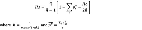
where ñ is the harmonic mean of nk (the number of individuals in each subpopulation), pki is the proportion (sometimes misleadingly called frequency) of allele i in subpopulation k.
-
Ht - Heterozygosity for the total population (Nei, 1987, pp. 164, eq. 7.40) is calculated as:
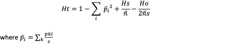
-
Dst - The average allele frequency differentiation between populations (Nei, 1987, pp. 163) is calculated as:

-
Htp - Unbiased estimate of Heterozygosity for the total population (Nei, 1987, pp. 165) is calculated as:

-
Dstp - Unbiased estimate of the average allele frequency differentiation between populations (Nei, 1987, pp. 165) is calculated as:
-
Fst - Measure of the extent of genetic differentiation of subpopulations (Nei, 1987, pp. 162, eq. 7.34) is calculated as:

-
Fstp - Unbiased measure of the extent of genetic differentiation of subpopulations (Nei, 1987, pp. 163, eq. 7.36) is calculated as:

-
Dest - Jost’s D (Jost, 2008, eq. 12) is calculated as:
-
Gst-max - The maximum level that Gst can obtain for the observed amount of genetic variation (Hedrick 2005, eq. 4a) is calculated as:

-
Gst-H - Gst standardized by the maximum level that it can obtain for the observed amount of genetic variation (Hedrick 2005, eq. 4b) is calculated as:

Confidence Intervals
The uncertainty of a parameter, in this case the mean of the statistic, can be summarised by a confidence interval (CI) which includes the true parameter value with a specified probability (i.e. confidence level; the parameter "conf" in this function).
In this function, CI are obtained using Bootstrap which is an inference method that samples with replacement the data (i.e. loci) and calculates the statistics every time.
This function uses the function boot (package boot) to perform the bootstrap replicates and the function boot.ci (package boot) to perform the calculations for the CI.
Four different types of nonparametric CI can be calculated (parameter "CI.type" in this function):
First order normal approximation interval ("norm").
Basic bootstrap interval ("basic").
Bootstrap percentile interval ("perc").
Adjusted bootstrap percentile interval ("bca").
The studentized bootstrap interval ("stud") was not included in the CI types because it is computationally intensive, it may produce estimates outside the range of plausible values and it has been found to be erratic in practice, see for example the "Studentized (t) Intervals" section in:
Nice tutorials about the different types of CI can be found in:
https://www.datacamp.com/tutorial/bootstrap-r
and
Efron and Tibshirani (1993, p. 162) and Davison and Hinkley (1997, p. 194) suggest that the number of bootstrap replicates should be between 1000 and 2000.
It is important to note that unreliable confidence intervals will be obtained if too few number of bootstrap replicates are used. Therefore, the function boot.ci will throw warnings and errors if bootstrap replicates are too few. Consider increasing then number of bootstrap replicates to at least 200.
The "bca" interval is often cited as the best for theoretical reasons, however it may produce unstable results if the bootstrap distribution is skewed or has extreme values. For example, you might get the warning "extreme order statistics used as endpoints" or the error "estimated adjustment 'a' is NA". In this case, you may want to use more bootstrap replicates or a different method or check your data for outliers.
The error "estimated adjustment 'w' is infinite" means that the estimated adjustment ‘w’ for the "bca" interval is infinite, which can happen when the empirical influence values are zero or very close to zero. This can be caused by various reasons, such as:
The number of bootstrap replicates is too small, the statistic of interest is constant or nearly constant across the bootstrap samples, the data contains outliers or extreme values.
You can try some possible solutions, such as:
Increasing the number of bootstrap replicates, using a different type of bootstrap confidence interval or removing or transforming the outliers or extreme values.
Plotting
The plot can be customised by including any parameter(s) from the function heatmap.2 (package gplots).
For the color palette you could try for example:
> library(viridis)
> res <- gl.report.fstat(platypus.gl, palette.divergent = viridis)
If a plot.file is given, the plot arising from this function is saved as an "RDS" binary file using the function saveRDS (package base); can be reloaded with function readRDS (package base). A file name must be specified for the plot to be saved.
If a plot directory (plot.dir) is specified, the gplot binary is saved to that directory; otherwise to the tempdir().
Your plot might not shown in full because your 'Plots' pane is too small (in RStudio). Increase the size of the 'Plots' pane before running the function. Alternatively, use the parameter 'plot.file' to save the plot to a file.
Parallelisation
If the parameter ncpus > 1, parallelisation is enabled. In Windows, parallel computing employs a "socket" approach that starts new copies of R on each core. POSIX systems, on the other hand (Mac, Linux, Unix, and BSD), utilise a "forking" approach that replicates the whole current version of R and transfers it to a new core.
Opening and terminating R sessions in each core involves a significant amount of processing time, therefore parallelisation in Windows machines is only quicker than not using parallelisation when nboots > 1000-2000.
Value
Two lists, the first list contains matrices with genetic statistics taken pairwise by population, the second list contains tables with the genetic statistics for each pair of populations. If nboots > 0, tables with the four statistics calculated with Low Confidence Intervals (LCI) and High Confidence Intervals (HCI).
Author(s)
Custodian: Luis Mijangos – Post to https://groups.google.com/d/forum/dartr
References
-
Alcala, N., & Rosenberg, N. A. (2017). Mathematical constraints on FST: Biallelic markers in arbitrarily many populations. Genetics (206), 1581-1600.
-
Berner, D. (2019). Allele frequency difference AFD–an intuitive alternative to FST for quantifying genetic population differentiation. Genes, 10(4), 308.
-
Davison AC, Hinkley DV (1997). Bootstrap Methods and their Application. Cambridge University Press: Cambridge.
-
Efron, B. (1979). Bootstrap methods: Another look at the jackknife. Annals of Statistics 7, 1–26.
-
Efron B, Tibshirani RJ (1993). An Introduction to the Bootstrap. Chapman and Hall: London.
-
Hedrick, P. W. (2005). A standardized genetic differentiation measure. Evolution, 59(8), 1633-1638.
-
Holsinger, K. E. (2012). Lecture notes in population genetics.
-
Holsinger, K. E., & Weir, B. S. (2009). Genetics in geographically structured populations: defining, estimating and interpreting FST. Nature Reviews Genetics, 10(9), 639- 650.
-
Jost, L. (2008). GST and its relatives do not measure differentiation. Molecular Ecology, 17(18), 4015-4026.
-
Meirmans, P. G., & Hedrick, P. W. (2011). Assessing population structure: FST and related measures. Molecular Ecology Resources, 11(1), 5-18.
-
Nei, M. (1987). Molecular evolutionary genetics: Columbia University Press.
-
Sherwin, W. B., Chao, A., Jost, L., & Smouse, P. E. (2017). Information theory broadens the spectrum of molecular ecology and evolution. Trends in Ecology & Evolution, 32(12), 948-963.
See Also
Other matched reports:
gl.mahal.assign(),
gl.report.bases(),
gl.report.factorloadings(),
gl.report.monomorphs()
Examples
res <- gl.report.fstat(platypus.gl)
Calculates the pairwise Hamming distance between DArT trimmed DNA sequences
Description
Hamming distance is calculated as the number of base differences between two sequences which can be expressed as a count or a proportion. Typically, it is calculated between two sequences of equal length. In the context of DArT trimmed sequences, which differ in length but which are anchored to the left by the restriction enzyme recognition sequence, it is sensible to compare the two trimmed sequences starting from immediately after the common recognition sequence and terminating at the last base of the shorter sequence.
Usage
gl.report.hamming(
  x,
  rs = 5,
  threshold = 3,
  tag.length = 69,
  plot.display = TRUE,
  plot.theme = theme_dartR(),
  plot.colors = NULL,
  plot.dir = NULL,
  plot.file = NULL,
  probar = FALSE,
  verbose = NULL
)
Arguments
x |
Name of the genlight object containing the SNP data [required]. |
rs |
Number of bases in the restriction enzyme recognition sequence [default 5]. |
threshold |
Minimum acceptable base pair difference for display on the boxplot and histogram [default 3]. |
tag.length |
Typical length of the sequence tags [default 69]. |
plot.display |
Specify if plot is to be produced [default TRUE]. |
plot.theme |
User specified theme [default theme_dartR()]. |
plot.colors |
Vector with two color names for the borders and fill [default c("#2171B5", "#6BAED6")]. |
plot.dir |
Directory to save the plot RDS files [default as specified by the global working directory or tempdir()] |
plot.file |
Filename (minus extension) for the RDS plot file [Required for plot save] |
probar |
If TRUE, a progress bar is displayed during run [defalut FALSE] |
verbose |
Verbosity: 0, silent or fatal errors; 1, begin and end; 2, progress log; 3, progress and results summary; 5, full report [default 2, unless specified using gl.set.verbosity]. |
Details
The function gl.filter.hamming will filter out one of
two loci if their Hamming distance is less than a specified percentage
Hamming distance can be computed by exploiting the fact that the dot product
of two binary vectors x and (1-y) counts the corresponding elements that are
different between x and y. This approach can also be used for vectors that
contain more than two possible values at each position (e.g. A, C, T or G).
If a pair of DNA sequences are of differing length, the longer is truncated.
The algorithm is that of Johann de Jong
https://johanndejong.wordpress.com/2015/10/02/faster-hamming-distance-in-r-2/
as implemented in utils.hamming
If plot.file is specified, plots are saved to the directory specified by the user, or the global
default working directory set by gl.set.wd() or to the tempdir().
Examples of other themes that can be used can be consulted in
Value
Returns unaltered genlight object
Author(s)
Custodian: Arthur Georges – Post to https://groups.google.com/d/forum/dartr
See Also
Other matched report:
gl.filter.excess.het(),
gl.report.allna(),
gl.report.callrate(),
gl.report.locmetric(),
gl.report.maf(),
gl.report.overshoot(),
gl.report.pa(),
gl.report.rdepth(),
gl.report.reproducibility(),
gl.report.secondaries(),
gl.report.taglength()
Examples
gl.report.hamming(testset.gl[,1:100])
gl.report.hamming(testset.gs[,1:100])

#' # SNP data
test <- platypus.gl
test <- gl.subsample.loc(platypus.gl,n=50)
result <- gl.report.hamming(test, verbose=3)
result <- gl.report.hamming(test, plot.file="ttest", verbose=3)
Reports observed, expected and unbiased heterozygosities and FIS (inbreeding coefficient) by population or by individual from SNP data
Description
Calculates the observed, expected and unbiased expected (i.e. corrected for sample size) heterozygosities and FIS (inbreeding coefficient) for each population or the observed heterozygosity for each individual in a genlight object.
Usage
gl.report.heterozygosity(
  x,
  method = "pop",
  n.invariant = 0,
  subsample.pop = FALSE,
  n.limit = 10,
  nboots = 0,
  boot.method = "ind",
  conf = 0.95,
  CI.type = "bca",
  ncpus = 1,
  plot.display = TRUE,
  plot.theme = theme_dartR(),
  plot.colors.pop = gl.colors("dis"),
  plot.colors.ind = gl.colors(2),
  plot.file = NULL,
  plot.dir = NULL,
  error.bar = "SD",
  verbose = NULL
)
Arguments
x |
Name of the genlight object containing the SNP data [required]. |
method |
Calculate heterozygosity by population (method='pop') or by individual (method='ind') [default 'pop']. |
n.invariant |
An estimate of the number of invariant sequence tags used to adjust the heterozygosity rate [default 0]. |
subsample.pop |
Whether subsample populations to estimate observed heterozygosity (see Details) [default FALSE]. |
n.limit |
Minimum number of individuals that should have a population to perform subsampling to estimate heterozygosity [default 10]. |
nboots |
Number of bootstrap replicates to obtain confidence intervals [default 0]. |
boot.method |
boostraping across individuals ("ind") or across loci ("loc") [default "ind"]. |
conf |
The confidence level of the required interval [default 0.95]. |
CI.type |
Method to estimate confidence intervals. One of "norm", "basic", "perc" or "bca" [default "bca"]. |
ncpus |
Number of processes to be used in parallel operation. If ncpus > 1 parallel operation is activated, see "Details" section [default 1]. |
plot.display |
Specify if plot is to be produced [default TRUE]. |
plot.theme |
Theme for the plot. See Details for options [default theme_dartR()]. |
plot.colors.pop |
A color palette for population plots or a list with as many colors as there are populations in the dataset [default gl.colors("dis")]. |
plot.colors.ind |
List of two color names for the borders and fill of the plot by individual [default gl.colors(2)]. |
plot.file |
Name for the RDS binary file to save (base name only, exclude extension) [default NULL]. |
plot.dir |
Directory to save the plot RDS files [default as specified by the global working directory or tempdir()]. |
error.bar |
Statistic to be plotted as error bar either "SD" (standard deviation) or "SE" (standard error) or "CI" (confidence intervals) [default "SD"]. |
verbose |
Verbosity: 0, silent or fatal errors; 1, begin and end; 2, progress log; 3, progress and results summary; 5, full report [default NULL, unless specified using gl.set.verbosity]. |
Details
Observed heterozygosity for a population takes the proportion of heterozygous loci for each individual and averages it over all individuals in that population. The calculations take into account missing values.
Expected heterozygosity for a population takes the expected proportion of heterozygotes, that is, expected under Hardy-Weinberg equilibrium, for each locus, then averages this across the loci for an average estimate for the population.
The unbiased expected heterozygosity is calculated using the correction for sample size following equation 2 from Nei 1978.
Accuracy of all heterozygosity estimates is affected by small sample sizes, and so is their comparison between populations or repeated analysis. Expected heterozygosities are less affected because their calculations are based on allele frequencies while observed heterozygosities are strongly susceptible to sampling effects when the sample size is small.
Observed heterozygosity for individuals is calculated as the proportion of loci that are heterozygous for that individual.
Finally, the loci that are invariant across all individuals in the dataset
(that is, across populations), is typically unknown. This can render
estimates of heterozygosity analysis specific, and so it is not valid to
compare such estimates across species or even across different analyses
(see Schimdt et al 2021). This is a similar problem faced by microsatellites.
If you have an estimate of the
number of invariant sequence tags (loci) in your data, such as provided by
gl.report.secondaries, you can specify it with the n.invariant
parameter to standardize your estimates of heterozygosity. This is called
autosomal heterozygosities by Schimddt et al (2021).
NOTE: It is important to realise that estimation of adjusted (autosomal) heterozygosity requires that secondaries not to be removed.
Heterozygosities and FIS (inbreeding coefficient) are calculated by locus within each population using the following equations, and then averaged across all loci:
Observed heterozygosity (Ho) = number of heterozygotes / n_Ind, where n_Ind is the number of individuals without missing data for that locus.
Observed heterozygosity adjusted (Ho.adj) <- Ho * n_Loc / (n_Loc + n.invariant), where n_Loc is the number of loci that do not have all missing data and n.invariant is an estimate of the number of invariant loci to adjust heterozygosity.
Expected heterozygosity (He) = 1 - (p^2 + q^2), where p is the frequency of the reference allele and q is the frequency of the alternative allele.
Expected heterozygosity adjusted (He.adj) = He * n_Loc / (n_Loc + n.invariant)
Unbiased expected heterozygosity (uHe) = He * (2 * n_Ind / (2 * n_Ind - 1))
Inbreeding coefficient (FIS) = 1 - Ho / uHe
Function's output
Output for method='pop' is an ordered barchart of observed heterozygosity, unbiased expected heterozygosity and FIS (Inbreeding coefficient) across populations together with a table of mean observed and expected heterozygosities and FIS by population and their respective standard deviations (SD). In the output, it is also reported by population: the number of loci used to estimate heterozygosity (n.Loc), the number of polymorphic loci (polyLoc), the number of monomorphic loci (monoLoc) and loci with all missing data (all_NALoc).
Output for method='ind' is a histogram and a boxplot of heterozygosity across individuals.
If a plot.file is given, the ggplot arising from this function is saved as an "RDS" binary file using saveRDS(); can be reloaded with readRDS(). A file name must be specified for the plot to be saved.
If a plot directory (plot.dir) is specified, the ggplot binary is saved to that directory; otherwise to the tempdir().
Examples of other themes that can be used can be consulted in:
Subsampling populations
To test the effect of five population sample sizes (n = 10, 5, 4, 3, 2) on observed heterozygosity estimates, the function subsamples individuals, without replacement. The subsampling is repeated 10 times for each sample size n. This approach is not an implementation of Schmidt et al (2021). Please refer to this paper for additional complexities in estimating heterozygosity using SNP data.
Error bars
The best method for presenting or assessing genetic statistics depends on the type of data you have and the specific questions you're trying to answer. Here's a brief overview of when you might use each method:
1. Confidence Intervals ("CI"):
- Usage: Often used to convey the precision of an estimate.
- Advantage: Confidence intervals give a range in which the true parameter (like a population mean) is likely to fall, given the data and a specified probability (like 95%).
- In Context: For genetic statistics, if you're estimating a parameter, a 95% CI gives you a range in which you're 95% confident the true parameter lies.
2. Standard Deviation ("SD"):
- Usage: Describes the amount of variation from the average in a set of data.
- Advantage: Allows for an understanding of the spread of individual data points around the mean.
- In Context: If you're looking at the distribution of a quantitative trait (like height) in a population with a particular genotype, the SD can describe how much individual heights vary around the average height.
3. Standard Error ("SE"):
- Usage: Describes the precision of the sample mean as an estimate of the population mean.
- Advantage: Smaller than the SD in large samples; it takes into account both the SD and the sample size.
- In Context: If you want to know how accurately your sample mean represents the population mean, you'd look at the SE.
Recommendation:
- If you're trying to convey the precision of an estimate, confidence intervals are very useful.
- For understanding variability within a sample, standard deviation is key.
- To see how well a sample mean might estimate a population mean, consider the standard error.
In practice, geneticists often use a combination of these methods to analyze and present their data, depending on their research questions and the nature of the data.
Confidence Intervals
The uncertainty of a parameter, in this case the mean of the statistic, can be summarised by a confidence interval (CI) which includes the true parameter value with a specified probability (i.e. confidence level; the parameter "conf" in this function).
In this function, CI are obtained using Bootstrap which is an inference method that samples with replacement the data (i.e. loci) and calculates the statistics every time.
This function uses the function boot (package boot) to perform the bootstrap replicates and the function boot.ci (package boot) to perform the calculations for the CI.
Four different types of nonparametric CI can be calculated (parameter "CI.type" in this function):
First order normal approximation interval ("norm").
Basic bootstrap interval ("basic").
Bootstrap percentile interval ("perc").
Adjusted bootstrap percentile interval ("bca").
The studentized bootstrap interval ("stud") was not included in the CI types because it is computationally intensive, it may produce estimates outside the range of plausible values and it has been found to be erratic in practice, see for example the "Studentized (t) Intervals" section in:
Nice tutorials about the different types of CI can be found in:
https://www.datacamp.com/tutorial/bootstrap-r
and
Efron and Tibshirani (1993, p. 162) and Davison and Hinkley (1997, p. 194) suggest that the number of bootstrap replicates should be between 1000 and 2000.
It is important to note that unreliable confidence intervals will be obtained if too few number of bootstrap replicates are used. Therefore, the function boot.ci will throw warnings and errors if bootstrap replicates are too few. Consider increasing the number of bootstrap replicates to at least 200.
The "bca" interval is often cited as the best for theoretical reasons, however it may produce unstable results if the bootstrap distribution is skewed or has extreme values. For example, you might get the warning "extreme order statistics used as endpoints" or the error "estimated adjustment 'a' is NA". In this case, you may want to use more bootstrap replicates or a different method or check your data for outliers.
The error "estimated adjustment 'w' is infinite" means that the estimated adjustment ‘w’ for the "bca" interval is infinite, which can happen when the empirical influence values are zero or very close to zero. This can be caused by various reasons, such as:
The number of bootstrap replicates is too small, the statistic of interest is constant or nearly constant across the bootstrap samples, the data contains outliers or extreme values.
You can try some possible solutions, such as:
Increasing the number of bootstrap replicates, using a different type of bootstrap confidence interval or removing or transforming the outliers or extreme values.
Parallelisation
If the parameter ncpus > 1, parallelisation is enabled. In Windows, parallel computing employs a "socket" approach that starts new copies of R on each core. POSIX systems, on the other hand (Mac, Linux, Unix, and BSD), utilise a "forking" approach that replicates the whole current version of R and transfers it to a new core.
Opening and terminating R sessions in each core involves a significant amount of processing time, therefore parallelisation in Windows machines is only quicker than not using parallelisation when nboots > 1000-2000.
Value
A dataframe containing population labels, heterozygosities, FIS, their standard deviations and sample sizes.
Author(s)
Custodian: Luis Mijangos (Post to https://groups.google.com/d/forum/dartr)
References
Nei, M. (1978). Estimation of average heterozygosity and genetic distance from a small number of individuals. Genetics, 89(3), 583-590.
Schmidt, T. L., Jasper, M. E., Weeks, A. R., & Hoffmann, A. A. (2021). Unbiased population heterozygosity estimates from genome‐wide sequence data. Methods in Ecology and Evolution, 12(10), 1888-1898.
See Also
Other unmatched report:
gl.allele.freq(),
gl.report.basics(),
gl.report.diversity(),
gl.report.excess.het(),
gl.report.polyploid_heterozygosity()
Examples
require("dartR.data")
df <- gl.report.heterozygosity(platypus.gl)
df <- gl.report.heterozygosity(platypus.gl,method='ind')
n.inv <- gl.report.secondaries(platypus.gl)
gl.report.heterozygosity(platypus.gl, n.invariant = n.inv[7, 2])
gl.report.heterozygosity(platypus.gl, subsample.pop = TRUE)

df <- gl.report.heterozygosity(platypus.gl)
Reports departure from Hardy-Weinberg proportions
Description
Calculates the probabilities of agreement with H-W proportions based on observed frequencies of reference homozygotes, heterozygotes and alternate homozygotes.
Usage
gl.report.hwe(
  x,
  subset = "each",
  method_sig = "Exact",
  multi_comp = FALSE,
  multi_comp_method = "BY",
  alpha_val = 0.05,
  pvalue_type = "midp",
  cc_val = 0.5,
  sig_only = TRUE,
  min_sample_size = 5,
  plot.out = TRUE,
  plot_colors = gl.colors("2c"),
  max_plots = 4,
  save2tmp = FALSE,
  verbose = NULL
)
Arguments
x |
Name of the genlight object containing the SNP data [required]. |
subset |
Whether to perform H-W tests within each population ("each"), or taking all individuals as one population ("all") (see details) [default 'each']. |
method_sig |
Method for determining statistical significance: 'ChiSquare' or 'Exact' [default 'Exact']. |
multi_comp |
Whether to adjust p-values for multiple comparisons [default FALSE]. |
multi_comp_method |
Method to adjust p-values for multiple comparisons: 'holm', 'hochberg', 'hommel', 'bonferroni', 'BH', 'BY', 'fdr' (see details) [default 'fdr']. |
alpha_val |
Level of significance for testing [default 0.05]. |
pvalue_type |
Type of p-value to be used in the Exact method. Either 'dost','selome','midp' (see details) [default 'midp']. |
cc_val |
The continuity correction applied to the ChiSquare test [default 0.5]. |
sig_only |
Whether the returned table should include loci with a significant departure from Hardy-Weinberg proportions [default TRUE]. |
min_sample_size |
Minimum number of individuals per population in which perform H-W tests [default 5]. |
plot.out |
If TRUE, will produce Ternary Plot(s) [default TRUE]. |
plot_colors |
Vector with two color names for the significant and not-significant loci [default gl.colors("2c")]. |
max_plots |
Maximum number of plots to print per page [default 4]. |
save2tmp |
If TRUE, saves any ggplots and listings to the session temporary directory (tempdir) [default FALSE]. |
verbose |
Verbosity: 0, silent or fatal errors; 1, begin and end; 2, progress log ; 3, progress and results summary; 5, full report [default NULL, unless specified using gl.set.verbosity]. |
Details
There are several factors that can cause deviations from Hardy-Weinberg proportions including: mutation, finite population size, selection, population structure, age structure, assortative mating, sex linkage, nonrandom sampling and genotyping errors. Therefore, testing for Hardy-Weinberg proportions should be a process that involves a careful evaluation of the results, a good place to start is Waples (2015). Note that tests for H-W proportions are only valid if there is no population substructure (assuming random mating) and have sufficient power only when there is sufficient sample size (n individuals > 15). Populations can be defined in three ways:
Merging all populations in the dataset using subset = 'all'.
Within each population separately using: subset = 'each'.
Within selected populations using for example: subset = c('pop1','pop2').
Two different statistical methods to test for deviations from Hardy Weinberg proportions:
The classical chi-square test (method_sig='ChiSquare') based on the function
HWChisqof the R package HardyWeinberg. By default a continuity correction is applied (cc_val=0.5). The continuity correction can be turned off (by specifying cc_val=0), for example in cases of extreme allele frequencies in which the continuity correction can lead to excessive type 1 error rates.The exact test (method_sig='Exact') based on the exact calculations contained in the function
HWExactStatsof the R package HardyWeinberg, and described in Wigginton et al. (2005). The exact test is recommended in most cases (Wigginton et al., 2005). Three different methods to estimate p-values (pvalue_type) in the Exact test can be used:'dost' p-value is computed as twice the tail area of a one-sided test.
'selome' p-value is computed as the sum of the probabilities of all samples less or equally likely as the current sample.
'midp', p-value is computed as half the probability of the current sample + the probabilities of all samples that are more extreme.
The standard exact p-value is overly conservative, in particular for small minor allele frequencies. The mid p-value ameliorates this problem by bringing the rejection rate closer to the nominal level, at the price of occasionally exceeding the nominal level (Graffelman & Moreno, 2013).
Correction for multiple tests can be applied using the following methods
based on the function p.adjust:
'holm' is also known as the sequential Bonferroni technique (Rice, 1989). This method has a greater statistical power than the standard Bonferroni test, however this method becomes very stringent when many tests are performed and many real deviations from the null hypothesis can go undetected (Waples, 2015).
'hochberg' based on Hochberg, 1988.
'hommel' based on Hommel, 1988. This method is more powerful than Hochberg's, but the difference is usually small.
'bonferroni' in which p-values are multiplied by the number of tests. This method is very stringent and therefore has reduced power to detect multiple departures from the null hypothesis.
'BH' based on Benjamini & Hochberg, 1995.
'BY' based on Benjamini & Yekutieli, 2001.
The first four methods are designed to give strong control of the family-wise
error rate. The last two methods control the false discovery rate (FDR),
the expected proportion of false discoveries among the rejected hypotheses.
The false discovery rate is a less stringent condition than the family-wise
error rate, so these methods are more powerful than the others, especially
when number of tests is large.
The number of tests on which the adjustment for multiple comparisons is
the number of populations times the number of loci.
Ternary plots
Ternary plots can be used to visualise patterns of H-W proportions (plot.out
= TRUE). P-values and the statistical (non)significance of a large number of
bi-allelic markers can be inferred from their position in a ternary plot.
See Graffelman & Morales-Camarena (2008) for further details. Ternary plots
are based on the function HWTernaryPlot from
the package HardyWeinberg. Each vertex of the Ternary plot represents one of
the three possible genotypes for SNP data: homozygous for the reference
allele (AA), heterozygous (AB) and homozygous for the alternative allele
(BB). Loci deviating significantly from Hardy-Weinberg proportions after
correction for multiple tests are shown in pink. The blue parabola
represents Hardy-Weinberg equilibrium, and the area between green lines
represents the acceptance region.
For these plots to work it is necessary to install the package ggtern.
Value
A dataframe containing loci, counts of reference SNP homozygotes, heterozygotes and alternate SNP homozygotes; probability of departure from H-W proportions, per locus significance with and without correction for multiple comparisons and the number of population where the same locus is significantly out of HWE.
Author(s)
Custodian: Luis Mijangos – Post to https://groups.google.com/d/forum/dartr
References
Benjamini, Y., and Yekutieli, D. (2001). The control of the false discovery rate in multiple testing under dependency. Annals of Statistics, 29, 1165–1188.
Graffelman, J. (2015). Exploring Diallelic Genetic Markers: The Hardy Weinberg Package. Journal of Statistical Software 64:1-23.
Graffelman, J. & Morales-Camarena, J. (2008). Graphical tests for Hardy-Weinberg equilibrium based on the ternary plot. Human Heredity 65:77-84.
Graffelman, J., & Moreno, V. (2013). The mid p-value in exact tests for Hardy-Weinberg equilibrium. Statistical applications in genetics and molecular biology, 12(4), 433-448.
Hochberg, Y. (1988). A sharper Bonferroni procedure for multiple tests of significance. Biometrika, 75, 800–803.
Hommel, G. (1988). A stagewise rejective multiple test procedure based on a modified Bonferroni test. Biometrika, 75, 383–386.
Rice, W. R. (1989). Analyzing tables of statistical tests. Evolution, 43(1), 223-225.
Waples, R. S. (2015). Testing for Hardy–Weinberg proportions: have we lost the plot?. Journal of heredity, 106(1), 1-19.
Wigginton, J.E., Cutler, D.J., & Abecasis, G.R. (2005). A Note on Exact Tests of Hardy-Weinberg Equilibrium. American Journal of Human Genetics 76:887-893.
See Also
Calculates pairwise population based Linkage Disequilibrium across all loci using the specified number of cores @family matched report
Description
This function is implemented in a parallel fashion to speed up the process.
There is also the ability to restart the function if crashed by specifying
the chunk file names or restarting the function exactly in the same way as in
the first run. This is implemented because sometimes, due to connectivity loss
between cores, the function may crash half way. Before running the function,
it is advisable to use the function gl.filter.allna to remove
loci with all missing data.
Usage
gl.report.ld(
  x,
  name = NULL,
  save = TRUE,
  outpath = tempdir(),
  nchunks = 2,
  ncores = 1,
  chunkname = NULL,
  probar = FALSE,
  verbose = NULL
)
Arguments
x |
A genlight or genind object created (genlight objects are internally
converted via |
name |
Character string for rdata file. If not given genind object name is used [default NULL]. |
save |
Switch if results are saved in a file [default TRUE]. |
outpath |
Folder where chunks and results are saved (if save=TRUE) [default tempdir()]. |
nchunks |
How many subchunks will be used (the less the faster, but if the routine crashes more bits are lost) [default 2]. |
ncores |
How many cores should be used [default 1]. |
chunkname |
The name of the chunks for saving [default NULL]. |
probar |
if TRUE, a progress bar is displayed for long loops [default = TRUE]. |
verbose |
Verbosity: 0, silent or fatal errors; 1, begin and end; 2, progress log; 3, progress and results summary; 5, full report [default 2 or as specified using gl.set.verbosity]. |
Value
Returns calculation of pairwise LD across all loci between subpopulations. This functions uses if specified many cores on your computer to speed up. And if save is used can restart (if save=TRUE is used) with the same command starting where it crashed. The final output is a data frame that holds all statistics of pairwise LD between loci. (See ?LD in package genetics for details).
Author(s)
Bernd Gruber (Post to https://groups.google.com/d/forum/dartr)
Calculates pairwise linkage disequilibrium by population
Description
This function calculates pairwise linkage disequilibrium (LD) by population
using the function ld from package snpStats.
If SNPs are not mapped to a reference genome, the parameter
ld.max.pairwise
should be set as NULL (the default). In this case, the
function will assign the same chromosome ("1") to all the SNPs in the dataset
and assign a sequence from 1 to n loci as the position of each SNP. The
function will then calculate LD for all possible SNP pair combinations.
If SNPs are mapped to a reference genome, the parameter
ld.max.pairwise
should be filled out (i.e. not NULL). In this case, the
information for SNP's position should be stored in the genlight accessor
"@position" and the SNP's chromosome name in the accessor "@chromosome"
(see examples). The function will then calculate LD within each chromosome
and for all possible SNP pair combinations within a distance of
ld.max.pairwise.
Usage
gl.report.ld.map(
  x,
  ld.max.pairwise = 1e+06,
  maf = 0.05,
  ld.stat = "R.squared",
  ind.limit = 10,
  stat.keep = "AvgPIC",
  ld.threshold.pops = 0.2,
  plot.display = TRUE,
  plot.theme = theme_dartR(),
  plot.file = NULL,
  plot.dir = NULL,
  histogram.colors = NULL,
  boxplot.colors = NULL,
  bins = 50,
  verbose = NULL
)
Arguments
x |
Name of the genlight object containing the SNP data [required]. |
ld.max.pairwise |
Maximum distance in number of base pairs at which LD should be calculated [default 1000000]. |
maf |
Minor allele frequency (by population) threshold to filter out loci. If a value > 1 is provided it will be interpreted as MAC (i.e. the minimum number of times an allele needs to be observed) [default 0.05]. |
ld.stat |
The LD measure to be calculated: "LLR", "OR", "Q", "Covar", "D.prime", "R.squared", and "R". See function ld from snpstats (package snpStats) for details [default "R.squared"]. |
ind.limit |
Minimum number of individuals that a population should contain to take it in account to report loci in LD [default 10]. |
stat.keep |
Name of the column from the slot |
ld.threshold.pops |
LD threshold to report in the plot of "Number of populations in which the same SNP pair are in LD" [default 0.2]. |
plot.display |
If TRUE, histograms of base composition are displayed in the plot window [default TRUE]. |
plot.theme |
Theme for the plot. See Details for options [default theme_dartR()]. |
plot.file |
Name for the RDS binary file to save (base name only, exclude extension) [default NULL] |
plot.dir |
Directory to save the plot RDS files [default as specified by the global working directory or tempdir()] |
histogram.colors |
Vector with two color names for the borders and fill [default NULL]. |
boxplot.colors |
A color palette for box plots by population or a list with as many colors as there are populations in the dataset [default NULL]. |
bins |
Number of bins to display in histograms [default 50]. |
verbose |
Verbosity: 0, silent or fatal errors; 1, begin and end; 2, progress log; 3, progress and results summary; 5, full report [default 2, unless specified using gl.set.verbosity]. |
Details
This function reports LD between SNP pairs by population.
The function gl.filter.ld filters out the SNPs in LD using as
input the results of gl.report.ld.map. The actual number of
SNPs to be filtered out depends on the parameters set in the function
gl.filter.ld.
Boxplots of LD by population and
a histogram showing LD frequency are presented.
Value
A dataframe with information for each SNP pair in LD.
Author(s)
Custodian: Luis Mijangos – Post to https://groups.google.com/d/forum/dartr
See Also
Other graphics:
gl.colors(),
gl.map.interactive(),
gl.plot.heatmap(),
gl.select.colors(),
gl.select.shapes(),
gl.smearplot(),
gl.tree.nj()
Examples
require("dartR.data")
x <- platypus.gl
x <- gl.filter.callrate(x,threshold = 1)
x <- gl.filter.monomorphs(x)
x$position <- x$other$loc.metrics$ChromPos_Platypus_Chrom_NCBIv1
x$chromosome <- as.factor(x$other$loc.metrics$Chrom_Platypus_Chrom_NCBIv1)
ld_res <- gl.report.ld.map(x,ld.max.pairwise = 10000000)
Reports summary of the slot $other$loc.metrics
Description
This function reports summary statistics (mean, minimum, average, quantiles), histograms
and boxplots for any loc.metric with numeric values (stored in
$other$loc.metrics) to assist the decision of choosing thresholds for the filter
function gl.filter.locmetric.
Usage
gl.report.locmetric(
  x,
  metric,
  plot.display = TRUE,
  plot.theme = theme_dartR(),
  plot.colors = NULL,
  plot.dir = NULL,
  plot.file = NULL,
  verbose = NULL
)
Arguments
x |
Name of the genlight object containing the SNP or presence/absence (SilicoDArT) data [required]. |
metric |
Name of the metric to be used for filtering [required]. |
plot.display |
Specify if plot is to be produced [default TRUE]. |
plot.theme |
User specified theme [default theme_dartR()]. |
plot.colors |
Vector with two color names for the borders and fill [default c("#2171B5", "#6BAED6")]. |
plot.dir |
Directory to save the plot RDS files [default as specified by the global working directory or tempdir()] |
plot.file |
Filename (minus extension) for the RDS plot file [Required for plot save] |
verbose |
Verbosity: 0, silent or fatal errors; 1, begin and end; 2, progress log; 3, progress and results summary; 5, full report [default NULL, unless specified using gl.set.verbosity]. |
Details
The function gl.filter.locmetric will filter out the
loci with a locmetric value below a specified threshold.
The fields that are included in dartR, and a short description, are found
below. Optionally, the user can also set his/her own field by adding a vector
into $other$loc.metrics as shown in the example. You can check the names of
all available loc.metrics via: names(gl$other$loc.metrics).
SnpPosition - position (zero is position 1) in the sequence tag of the defined SNP variant base.
CallRate - proportion of samples for which the genotype call is non-missing (that is, not '-' ).
OneRatioRef - proportion of samples for which the genotype score is 0.
OneRatioSnp - proportion of samples for which the genotype score is 2.
FreqHomRef - proportion of samples homozygous for the Reference allele.
FreqHomSnp - proportion of samples homozygous for the Alternate (SNP) allele.
FreqHets - proportion of samples which score as heterozygous, that is, scored as 1.
PICRef - polymorphism information content (PIC) for the Reference allele.
PICSnp - polymorphism information content (PIC) for the SNP.
AvgPIC - average of the polymorphism information content (PIC) of the reference and SNP alleles.
AvgCountRef - sum of the tag read counts for all samples, divided by the number of samples with non-zero tag read counts, for the Reference allele row.
AvgCountSnp - sum of the tag read counts for all samples, divided by the number of samples with non-zero tag read counts, for the Alternate (SNP) allele row.
RepAvg - proportion of technical replicate assay pairs for which the marker score is consistent.
rdepth - read depth.
Function's output The minimum, maximum, mean and a tabulation of quantiles of the locmetric values against thresholds rate are provided. Output also includes a boxplot and a histogram. Quantiles are partitions of a finite set of values into q subsets of (nearly) equal sizes. In this function q = 20. Quantiles are useful measures because they are less susceptible to long-tailed distributions and outliers. Plot colours can be set with gl.select.colors(). If plot.file is specified, plots are saved to the directory specified by the user, or the global default working directory set by gl.set.wd() or to the tempdir(). Examples of other themes that can be used can be consulted in:
Value
An unaltered genlight object.
Author(s)
Luis Mijangos (Post to https://groups.google.com/d/forum/dartr)
See Also
Other matched report:
gl.filter.excess.het(),
gl.report.allna(),
gl.report.callrate(),
gl.report.hamming(),
gl.report.maf(),
gl.report.overshoot(),
gl.report.pa(),
gl.report.rdepth(),
gl.report.reproducibility(),
gl.report.secondaries(),
gl.report.taglength()
Examples
# SNP data
out <- gl.report.locmetric(testset.gl,metric='SnpPosition')
# Tag P/A data
out <- gl.report.locmetric(testset.gs,metric='AvgReadDepth')
Reports minor allele frequency (MAF) for each locus in a SNP dataset
Description
This script provides summary histograms of MAF for each
population and an overall histogram to assist the decision of
choosing thresholds for the filter function gl.filter.maf
Usage
gl.report.maf(
  x,
  as.pop = NULL,
  maf.limit = 0.5,
  ind.limit = 5,
  plot.display = TRUE,
  plot.theme = theme_dartR(),
  plot.colors = NULL,
  plot.dir = NULL,
  plot.file = NULL,
  bins = 25,
  verbose = NULL
)
Arguments
x |
Name of the genlight object containing the SNP data [required]. |
as.pop |
Temporarily assign another locus metric as the population for the purposes of deletions [default NULL]. |
maf.limit |
Show histograms MAF range <= maf.limit [default 0.5]. |
ind.limit |
Show histograms only for populations of size greater than ind.limit [default 5]. |
plot.display |
Specify if plot is to be displayed in the graphics window [default TRUE]. |
plot.theme |
User specified theme [default theme_dartR()]. |
plot.colors |
Vector with color names for the borders and fill [default c("#2171B5", "#6BAED6")]. |
plot.dir |
Directory to save the plot RDS files [default as specified by the global working directory or tempdir()] |
plot.file |
Filename (minus extension) for the RDS plot file [Required for plot save]. |
bins |
Number of bins to display in histograms [default 25]. |
verbose |
Verbosity: 0, silent or fatal errors; 1, begin and end; 2, progress log ; 3, progress and results summary; 5, full report [default NULL, unless specified using gl.set.verbosity]. |
Details
The function gl.filter.maf will filter out the loci with MAF
below a specified threshold.
Function's output
The minimum, maximum, mean and a tabulation of MAF quantiles against thresholds rate are provided. Output also includes a boxplot and a histogram.
This function reports the MAF for each of several quantiles. Quantiles are partitions of a finite set of values into q subsets of (nearly) equal sizes. In this function q = 20. Quantiles are useful measures because they are less susceptible to long-tailed distributions and outliers.
Plot colours can be set with gl.select.colors().
If plot.file is specified, plots are saved to the directory specified by the user, or the global default working directory set by gl.set.wd() or to the tempdir().
Examples of other themes that can be used can be consulted in
Value
An unaltered genlight object
Author(s)
Custodian: Arthur Georges (Post to https://groups.google.com/d/forum/dartr)
See Also
Other matched report:
gl.filter.excess.het(),
gl.report.allna(),
gl.report.callrate(),
gl.report.hamming(),
gl.report.locmetric(),
gl.report.overshoot(),
gl.report.pa(),
gl.report.rdepth(),
gl.report.reproducibility(),
gl.report.secondaries(),
gl.report.taglength()
Examples
gl <- gl.filter.allna(platypus.gl)
gl.report.maf(gl)
Reports monomorphic loci
Description
This script reports the number of monomorphic loci and those with all NAs in a genlight {adegenet} object
Usage
gl.report.monomorphs(x, verbose = NULL)
Arguments
x |
Name of the input genlight object [required]. |
verbose |
Verbosity: 0, silent or fatal errors; 1, begin and end; 2, progress log; 3, progress and results summary; 5, full report [default NULL, unless specified using gl.set.verbosity]. |
Details
A DArT dataset will not have monomorphic loci, but they can arise, along with loci that are scored all NA, when populations or individuals are deleted. Retaining monomorphic loci unnecessarily increases the size of the dataset and will affect some calculations. Note that for SNP data, NAs likely represent null alleles; in tag presence/absence data, NAs represent missing values (presence/absence could not be reliably scored)
Value
An unaltered genlight object
Author(s)
Custodian: Arthur Georges – Post to https://groups.google.com/d/forum/dartr
See Also
Other matched reports:
gl.mahal.assign(),
gl.report.bases(),
gl.report.factorloadings(),
gl.report.fstat()
Examples
# SNP data
  gl.report.monomorphs(testset.gl)
# SilicoDArT data
  gl.report.monomorphs(testset.gs)
Reports loci for which the SNP has been trimmed from the sequence tag along with the adaptor
Description
This function checks the position of the SNP within the trimmed sequence tag and identifies those for which the SNP position is outside the trimmed sequence tag. This can happen, rarely, when the sequence containing the SNP resembles the adaptor.
Usage
gl.report.overshoot(x, verbose = NULL)
Arguments
x |
Name of the genlight object [required]. |
verbose |
Verbosity: 0, silent or fatal errors; 1, begin and end; 2, progress log; 3, progress and results summary; 5, full report [default NULL, unless specified using gl.set.verbosity]. |
Details
The SNP genotype can still be used in most analyses, but functions like gl2fasta() will present challenges if the SNP has been trimmed from the sequence tag. Resultant ggplot(s) and the tabulation(s) are saved to the session's temporary directory.
Value
An unaltered genlight object
Author(s)
Custodian: Arthur Georges – Post to https://groups.google.com/d/forum/dartr
See Also
Other matched report:
gl.filter.excess.het(),
gl.report.allna(),
gl.report.callrate(),
gl.report.hamming(),
gl.report.locmetric(),
gl.report.maf(),
gl.report.pa(),
gl.report.rdepth(),
gl.report.reproducibility(),
gl.report.secondaries(),
gl.report.taglength()
Examples
gl.report.overshoot(testset.gl)
Reports private alleles (and fixed alleles) per pair of populations
Description
This function reports private alleles in one population compared with a second population, for all populations taken pairwise. It also reports a count of fixed allelic differences and the mean absolute allele frequency differences (AFD) between pairs of populations.
Usage
gl.report.pa(
  x,
  x2 = NULL,
  method = "pairwise",
  loc.names = FALSE,
  test.asym = FALSE,
  test.asym.boot = 100,
  plot.display = FALSE,
  matrix.pa = FALSE,
  plot.font = 14,
  map.interactive = FALSE,
  provider = "Esri.NatGeoWorldMap",
  palette.discrete = NULL,
  plot.file = NULL,
  plot.dir = NULL,
  verbose = NULL
)
Arguments
x |
Name of the genlight object containing the SNP or SilicoDArT data [required]. |
x2 |
If two separate genlight objects are to be compared this can be provided here, but they must have the same number of SNPs [default NULL]. |
method |
Method to calculate private alleles: 'pairwise' comparison or compare each population against the rest 'one2rest' [default 'pairwise']. |
loc.names |
Whether names of loci with private alleles and fixed differences should reported. If TRUE, loci names are reported using a list |
test.asym |
Bootstrap test for significant differences of private alleles (see details section) [default FALSE]. |
test.asym.boot |
Number of bootstraps [default 100]. [default FALSE]. |
plot.display |
Specify if Sankey plot is to be produced [default FALSE]. |
matrix.pa |
Whether to generate a matrix of private alleles [default FALSE]. |
plot.font |
Numeric font size in pixels for the node text labels [default 14]. |
map.interactive |
Specify whether an interactive map showing private alleles between populations is to be produced [default FALSE]. |
provider |
Passed to leaflet [default "Esri.NatGeoWorldMap"]. |
palette.discrete |
A discrete palette for the color of populations or a list with as many colors as there are populations in the dataset [default gl.select.colors(x)]. |
plot.file |
Name for the RDS binary file to save (base name only, exclude extension) [default NULL] |
plot.dir |
Directory in which to save files [default = working directory] |
verbose |
Verbosity: 0, silent, fatal errors only; 1, flag function begin and end; 2, progress log; 3, progress and results summary; 5, full report [default 2 or as specified using gl.set.verbosity]. |
Details
Note that the number of paired alleles between two populations is not a symmetric dissimilarity measure.
If no x2 is provided, the function uses the pop(gl) hierarchy to determine pairs of populations, otherwise it runs a single comparison between x and x2.
Hint: in case you want to run comparisons between individuals (assuming individual names are unique), you can simply redefine your population names with your individual names, as below:
pop(gl) <- indNames(gl)
Definition of fixed and private alleles
The table below shows the possible cases of allele frequencies between two populations (0 = homozygote for Allele 1, x = both Alleles are present, 1 = homozygote for Allele 2).
p: cases where there is a private allele in pop1 compared to pop2 (but not viceversa)
f: cases where there is a fixed allele in pop1 (and pop2, as those cases are symmetric)
| pop1 | ||||
| 0 | x | 1 | ||
| 0 | - | p | p,f | |
| pop2 | x | - | - | - |
| 1 | p,f | p | - | |
The absolute allele frequency difference (AFD) in this function is a simple differentiation metric displaying intuitive properties which provides a valuable alternative to FST. For details about its properties and how it is calculated see Berner (2019).
The Bootstrap test for significant differences of private alleles uses a bootstrap simulation by shuffling individuals between a pair of populations and drawing with replacement. For each bootstrap the ratio of private alleles is compared to the actual ratio and recorded how often it is larger than the simulated one. If number of individuals are different between population bootstrap is done using the smaller number of samples in both populations.
The function also reports an estimation of the lower bound of the number of undetected private alleles using the Good-Turing frequency formula, originally developed for cryptography, which estimates in an ecological context the true frequencies of rare species in a single assemblage based on an incomplete sample of individuals. The approach is described in Chao et al. (2017). For this function, the equation 2c is used. This estimate is reported in the output table as Chao1 and Chao2.
In this function a Sankey Diagram is used to visualize patterns of private alleles between populations. This diagram allows to display flows (private alleles) between nodes (populations). Their links are represented with arcs that have a width proportional to the importance of the flow (number of private alleles).
if save2temp=TRUE, resultant plot(s) and the tabulation(s) are saved to the session's temporary directory.
Value
A data.frame. Each row shows, for each pair of populations the number of individuals in each population, the number of loci with fixed differences (same for both populations) in pop1 (compared to pop2) and viceversa. Same for private alleles and finally the absolute mean allele frequency difference between loci (AFD). If loc.names = TRUE, loci names with private alleles and fixed differences are reported in a list in addition to the dataframe.
Author(s)
Custodian: Bernd Gruber – Post to https://groups.google.com/d/forum/dartr
References
Berner, D. (2019). Allele frequency difference AFD – an intuitive alternative to FST for quantifying genetic population differentiation. Genes, 10(4), 308.
Chao, Anne, et al. "Deciphering the enigma of undetected species, phylogenetic, and functional diversity based on Good-Turing theory." Ecology 98.11 (2017): 2914-2929.
See Also
Other matched report:
gl.filter.excess.het(),
gl.report.allna(),
gl.report.callrate(),
gl.report.hamming(),
gl.report.locmetric(),
gl.report.maf(),
gl.report.overshoot(),
gl.report.rdepth(),
gl.report.reproducibility(),
gl.report.secondaries(),
gl.report.taglength()
Other report functions:
gl.report.replicates()
Examples
out <- gl.report.pa(platypus.gl)

out <- gl.report.pa(platypus.gl)
Reports observed, expected and unbiased heterozygosities and FIS (inbreeding coefficient) by population or by individual from SNP data
Description
Calculates the observed, expected and unbiased expected (i.e. corrected for sample size) heterozygosities and FIS (inbreeding coefficient) for each population or the observed heterozygosity for each individual in a genlight object.
Usage
gl.report.polyploid_heterozygosity(
  x,
  method = "pop",
  n.invariant = 0,
  subsample.pop = FALSE,
  n.limit = 10,
  nboots = 0,
  conf = 0.95,
  CI.type = "bca",
  ncpus = 1,
  plot.display = TRUE,
  plot.theme = theme_dartR(),
  plot.colors.pop = gl.colors("dis"),
  plot.colors.ind = gl.colors(2),
  plot.file = NULL,
  plot.dir = NULL,
  error.bar = "SD",
  verbose = NULL
)
Arguments
x |
Name of the genlight object containing the SNP data that converted to dosage mode [required]. |
method |
Calculate heterozygosity by population (method='pop') or by individual (method='ind') [default 'pop']. |
n.invariant |
An estimate of the number of invariant sequence tags used to adjust the heterozygosity rate [default 0]. |
subsample.pop |
Whether subsample populations to estimate observed heterozygosity (see Details) [default FALSE]. |
n.limit |
Minimum number of individuals that should have a population to perform subsampling to estimate heterozygosity [default 10]. |
nboots |
Number of bootstrap replicates to obtain confidence intervals [default 0]. |
conf |
The confidence level of the required interval [default 0.95]. |
CI.type |
Method to estimate confidence intervals. One of "norm", "basic", "perc" or "bca" [default "bca"]. |
ncpus |
Number of processes to be used in parallel operation. If ncpus > 1 parallel operation is activated, see "Details" section [default 1]. |
plot.display |
Specify if plot is to be produced [default TRUE]. |
plot.theme |
Theme for the plot. See Details for options [default theme_dartR()]. |
plot.colors.pop |
A color palette for population plots or a list with as many colors as there are populations in the dataset [default gl.colors("dis")]. |
plot.colors.ind |
List of two color names for the borders and fill of the plot by individual [default gl.colors(2)]. |
plot.file |
Name for the RDS binary file to save (base name only, exclude extension) [default NULL]. |
plot.dir |
Directory to save the plot RDS files [default as specified by the global working directory or tempdir()]. |
error.bar |
Statistic to be plotted as error bar either "SD" (standard deviation) or "SE" (standard error) or "CI" (confidence intervals) [default "SD"]. |
verbose |
Verbosity: 0, silent or fatal errors; 1, begin and end; 2, progress log; 3, progress and results summary; 5, full report [default NULL, unless specified using gl.set.verbosity]. |
Details
Observed heterozygosity for a population takes the proportion of heterozygous loci for each individual and averages it over all individuals in that population. The calculations take into account missing values.
Expected heterozygosity for a population takes the expected proportion of heterozygotes, that is, expected under Hardy-Weinberg equilibrium, for each locus, then averages this across the loci for an average estimate for the population.
The unbiased expected heterozygosity is calculated using the correction for sample size following equation 2 from Nei 1978.
Accuracy of all heterozygosity estimates is affected by small sample sizes, and so is their comparison between populations or repeated analysis. Expected heterozygosities are less affected because their calculations are based on allele frequencies while observed heterozygosities are strongly susceptible to sampling effects when the sample size is small.
Observed heterozygosity for individuals is calculated as the proportion of heterozygous gametes that could be produced by that individual.
Finally, the loci that are invariant across all individuals in the dataset
(that is, across populations), is typically unknown. This can render
estimates of heterozygosity analysis specific, and so it is not valid to
compare such estimates across species or even across different analyses
(see Schimdt et al 2021). This is a similar problem faced by microsatellites.
If you have an estimate of the
number of invariant sequence tags (loci) in your data, such as provided by
gl.report.secondaries, you can specify it with the n.invariant
parameter to standardize your estimates of heterozygosity. This is called
autosomal heterozygosities by Schimddt et al (2021).
NOTE: It is important to realise that estimation of adjusted (autosomal) heterozygosity requires that secondaries not to be removed.
Heterozygosities and FIS (inbreeding coefficient) are calculated by locus within each population using the following equations, and then averaged across all loci:
Observed heterozygosity (Ho) = number of heterozygous gametes / all combinations of gametes, where n_Ind is the number of individuals without missing data for that locus.
Observed heterozygosity adjusted (Ho.adj) <- Ho * n_Loc / (n_Loc + n.invariant), where n_Loc is the number of loci that do not have all missing data and n.invariant is an estimate of the number of invariant loci to adjust heterozygosity.
Expected heterozygosity (He) = 1 - (p^2 + q^2), where p is the frequency of the reference allele and q is the frequency of the alternative allele.
Expected heterozygosity adjusted (He.adj) = He * n_Loc / (n_Loc + n.invariant)
Unbiased expected heterozygosity (uHe) = He * (2 * n_Ind / (2 * n_Ind - 1))
Inbreeding coefficient (FIS) = 1 - Ho / uHe
Function's output
Output for method='pop' is an ordered barchart of observed heterozygosity, unbiased expected heterozygosity and FIS (Inbreeding coefficient) across populations together with a table of mean observed and expected heterozygosities and FIS by population and their respective standard deviations (SD). In the output, it is also reported by population: the number of loci used to estimate heterozygosity (n.Loc), the number of polymorphic loci (polyLoc), the number of monomorphic loci (monoLoc) and loci with all missing data (all_NALoc).
Output for method='ind' is a histogram and a boxplot of heterozygosity across individuals.
If a plot.file is given, the ggplot arising from this function is saved as an "RDS" binary file using saveRDS(); can be reloaded with readRDS(). A file name must be specified for the plot to be saved.
If a plot directory (plot.dir) is specified, the ggplot binary is saved to that directory; otherwise to the tempdir().
Examples of other themes that can be used can be consulted in:
Subsampling populations
To test the effect of five population sample sizes (n = 10, 5, 4, 3, 2) on observed heterozygosity estimates, the function subsamples individuals, without replacement. The subsampling is repeated 10 times for each sample size n. This approach is an implementation of Schmidt et al (2021).
Error bars
The best method for presenting or assessing genetic statistics depends on the type of data you have and the specific questions you're trying to answer. Here's a brief overview of when you might use each method:
1. Confidence Intervals ("CI"):
- Usage: Often used to convey the precision of an estimate.
- Advantage: Confidence intervals give a range in which the true parameter (like a population mean) is likely to fall, given the data and a specified probability (like 95%).
- In Context: For genetic statistics, if you're estimating a parameter, a 95% CI gives you a range in which you're 95% confident the true parameter lies.
2. Standard Deviation ("SD"):
- Usage: Describes the amount of variation from the average in a set of data.
- Advantage: Allows for an understanding of the spread of individual data points around the mean.
- In Context: If you're looking at the distribution of a quantitative trait (like height) in a population with a particular genotype, the SD can describe how much individual heights vary around the average height.
3. Standard Error ("SE"):
- Usage: Describes the precision of the sample mean as an estimate of the population mean.
- Advantage: Smaller than the SD in large samples; it takes into account both the SD and the sample size.
- In Context: If you want to know how accurately your sample mean represents the population mean, you'd look at the SE.
Recommendation:
- If you're trying to convey the precision of an estimate, confidence intervals are very useful.
- For understanding variability within a sample, standard deviation is key.
- To see how well a sample mean might estimate a population mean, consider the standard error.
analyze and present their data, depending on their research questions and the nature of the data.
Confidence Intervals
The uncertainty of a parameter, in this case the mean of the statistic, can be summarised by a confidence interval (CI) which includes the true parameter value with a specified probability (i.e. confidence level; the parameter "conf" in this function).
In this function, CI are obtained using Bootstrap which is an inference method that samples with replacement the data (i.e. loci) and calculates the statistics every time.
This function uses the function boot (package boot) to perform the bootstrap replicates and the function boot.ci (package boot) to perform the calculations for the CI.
Four different types of nonparametric CI can be calculated (parameter "CI.type" in this function):
First order normal approximation interval ("norm").
Basic bootstrap interval ("basic").
Bootstrap percentile interval ("perc").
Adjusted bootstrap percentile interval ("bca").
The studentized bootstrap interval ("stud") was not included in the CI types because it is computationally intensive, it may produce estimates outside the range of plausible values and it has been found to be erratic in practice, see for example the "Studentized (t) Intervals" section in:
Nice tutorials about the different types of CI can be found in:
https://www.datacamp.com/tutorial/bootstrap-r
and
Efron and Tibshirani (1993, p. 162) and Davison and Hinkley (1997, p. 194) suggest that the number of bootstrap replicates should be between 1000 and 2000.
It is important to note that unreliable confidence intervals will be obtained if too few number of bootstrap replicates are used. Therefore, the function boot.ci will throw warnings and errors if bootstrap replicates are too few. Consider increasing the number of bootstrap replicates to at least 200.
The "bca" interval is often cited as the best for theoretical reasons, however it may produce unstable results if the bootstrap distribution is skewed or has extreme values. For example, you might get the warning "extreme order statistics used as endpoints" or the error "estimated adjustment 'a' is NA". In this case, you may want to use more bootstrap replicates or a different method or check your data for outliers.
The error "estimated adjustment 'w' is infinite" means that the estimated adjustment ‘w’ for the "bca" interval is infinite, which can happen when the empirical influence values are zero or very close to zero. This can be caused by various reasons, such as:
The number of bootstrap replicates is too small, the statistic of interest is constant or nearly constant across the bootstrap samples, the data contains outliers or extreme values.
You can try some possible solutions, such as:
Increasing the number of bootstrap replicates, using a different type of bootstrap confidence interval or removing or transforming the outliers or extreme values.
Parallelisation
If the parameter ncpus > 1, parallelisation is enabled. In Windows, parallel computing employs a "socket" approach that starts new copies of R on each core. POSIX systems, on the other hand (Mac, Linux, Unix, and BSD), utilise a "forking" approach that replicates the whole current version of R and transfers it to a new core.
Opening and terminating R sessions in each core involves a significant amount of processing time, therefore parallelisation in Windows machines is only quicker than not using parallelisation when nboots > 1000-2000.
Value
A dataframe containing population labels, heterozygosities, FIS, their standard deviations and sample sizes.
Author(s)
Custodian: Ching Ching Lau (Post to https://groups.google.com/d/forum/dartr)
References
Moody, M. E., Mueller, L. D., & Soltis, D. E. (1993). Genetic variation and random drift in autotetraploid populations. Genetics, 134(2), 649-657.
See Also
Other unmatched report:
gl.allele.freq(),
gl.report.basics(),
gl.report.diversity(),
gl.report.excess.het(),
gl.report.heterozygosity()
Reports summary of Read Depth for each locus
Description
SNP datasets generated by DArT report AvgCountRef and AvgCountSnp as counts of sequence tags for the reference and alternate alleles respectively. These can be used to back calculate Read Depth. Fragment presence/absence datasets as provided by DArT (SilicoDArT) provide Average Read Depth and Standard Deviation of Read Depth as standard columns in their report. This function reports the read depth by locus for each of several quantiles.
Usage
gl.report.rdepth(
  x,
  plot.display = TRUE,
  plot.theme = theme_dartR(),
  plot.colors = NULL,
  plot.dir = NULL,
  plot.file = NULL,
  verbose = NULL
)
Arguments
x |
Name of the genlight object containing the SNP or presence/absence (SilicoDArT) data [required]. |
plot.display |
Specify if plot is to be produced [default TRUE]. |
plot.theme |
User specified theme [default theme_dartR()]. |
plot.colors |
Vector with two color names for the borders and fill [default c("#2171B5", "#6BAED6")]. |
plot.dir |
Directory to save the plot RDS files [default as specified by the global working directory or tempdir()] |
plot.file |
Filename (minus extension) for the RDS plot file [Required for plot save] |
verbose |
Verbosity: 0, silent or fatal errors; 1, begin and end; 2, progress log; 3, progress and results summary; 5, full report [default 2, unless specified using gl.set.verbosity]. |
Details
The function displays a table of minimum, maximum, mean and quantiles for
read depth against possible thresholds that might subsequently be specified
in gl.filter.rdepth. If plot.display=TRUE, display also includes a
boxplot and a histogram to guide in the selection of a threshold for
filtering on read depth.
Plot colours can be set with gl.select.colors().
If plot.file is specified, plots are saved to the directory specified by the user, or the global
default working directory set by gl.set.wd() or to the tempdir().
For examples of themes, see
Value
An unaltered genlight object
Author(s)
Custodian: Arthur Georges – Post to https://groups.google.com/d/forum/dartr
See Also
Other matched report:
gl.filter.excess.het(),
gl.report.allna(),
gl.report.callrate(),
gl.report.hamming(),
gl.report.locmetric(),
gl.report.maf(),
gl.report.overshoot(),
gl.report.pa(),
gl.report.reproducibility(),
gl.report.secondaries(),
gl.report.taglength()
Examples
# SNP data
df <- gl.report.rdepth(testset.gl)
df <- gl.report.rdepth(testset.gs)
Identify replicated individuals
Description
Identify replicated individuals
Usage
gl.report.replicates(
  x,
  loc_threshold = 100,
  perc_geno = 0.95,
  plot.out = TRUE,
  plot_theme = theme_dartR(),
  plot_colors = c("#2171B5", "#6BAED6"),
  bins = 100,
  verbose = NULL
)
Arguments
x |
Name of the genlight object containing the SNP data [required]. |
loc_threshold |
Minimum number of loci required to asses that two individuals are replicates [default 100]. |
perc_geno |
Mimimum percentage of genotypes in which two individuals should be the same [default 0.95]. |
plot.out |
Specify if plot is to be produced [default TRUE]. |
plot_theme |
User specified theme [default theme_dartR()]. |
plot_colors |
Vector with two color names for the borders and fill [default c("#2171B5", "#6BAED6")]. |
bins |
Number of bins to display in histograms [default 100]. |
verbose |
Verbosity: 0, silent or fatal errors; 1, begin and end; 2, progress log; 3, progress and results summary; 5, full report [default 2, unless specified using gl.set.verbosity]. |
Details
This function uses an C++ implementation, so package Rcpp needs to be installed and it is therefore fast (once it has compiled the function after the first run).
Ideally, in a large dataset with related and unrelated individuals and several replicated individuals, such as in a capture/mark/recapture study, the first histogram should have four "peaks". The first peak should represent unrelated individuals, the second peak should correspond to second-degree relationships (such as cousins), the third peak should represent first-degree relationships (like parent/offspring and full siblings), and the fourth peak should represent replicated individuals.
In order to ensure that replicated individuals are properly identified, it's important to have a clear separation between the third and fourth peaks in the second histogram. This means that there should be bins with zero counts between these two peaks.
Value
A list with three elements:
table.rep: A dataframe with pairwise results of percentage of same genotypes between two individuals, the number of loci used in the comparison and the missing data for each individual.
ind.list.drop: A vector of replicated individuals to be dropped. Replicated individual with the least missing data is reported.
ind.list.rep: A list of of each individual that has replicates in the dataset, the name of the replicates and the percentage of the same genotype.
Author(s)
Custodian: Luis Mijangos – Post to https://groups.google.com/d/forum/dartr
See Also
Other report functions:
gl.report.pa()
Examples
res_rep <- gl.report.replicates(platypus.gl, loc_threshold = 500,
perc_geno = 0.85)
Reports summary of RepAvg (repeatability averaged over both alleles for each locus) or reproducibility (repeatability of the scores for fragment presence/absence)
Description
SNP datasets generated by DArT have an index, RepAvg, generated by reproducing the data independently for 30 of alleles that give a repeatable result, averaged over both alleles for each locus. In the case of fragment presence/absence data (SilicoDArT), repeatability is the percentage of scores that are repeated in the technical replicate dataset.
Usage
gl.report.reproducibility(
  x,
  plot.display = TRUE,
  plot.theme = theme_dartR(),
  plot.colors = NULL,
  plot.dir = NULL,
  plot.file = NULL,
  verbose = NULL
)
Arguments
x |
Name of the genlight object containing the SNP or presence/absence (SilicoDArT) data [required]. |
plot.display |
Specify if plot is to be produced [default TRUE]. |
plot.theme |
Theme for the plot. See Details for options [default theme_dartR()]. |
plot.colors |
Vector with two color names for the borders and fill [default c("#2171B5", "#6BAED6")]. |
plot.dir |
Directory to save the plot RDS files [default as specified by the global working directory or tempdir()] |
plot.file |
Filename (minus extension) for the RDS plot file [Required for plot save] |
verbose |
Verbosity: 0, silent or fatal errors; 1, begin and end; 2, progress log; 3, progress and results summary; 5, full report [default 2, unless specified using gl.set.verbosity]. |
Details
The function displays a table of minimum, maximum, mean and quantiles for
repeatbility against possible thresholds that might subsequently be
specified in gl.filter.reproducibility.
If plot.display=TRUE, display also includes a boxplot and a histogram to guide
in the selection of a threshold for filtering on repeatability.
If plot.file is specified, plots are saved to the directory specified by the user, or the global
default working directory set by gl.set.wd() or to the tempdir().
For examples of themes, see:
Value
An unaltered genlight object
Author(s)
Custodian: Arthur Georges – Post to https://groups.google.com/d/forum/dartr
See Also
Other matched report:
gl.filter.excess.het(),
gl.report.allna(),
gl.report.callrate(),
gl.report.hamming(),
gl.report.locmetric(),
gl.report.maf(),
gl.report.overshoot(),
gl.report.pa(),
gl.report.rdepth(),
gl.report.secondaries(),
gl.report.taglength()
Examples
# SNP data
  out <- gl.report.reproducibility(testset.gl)

# Tag P/A data
  out <- gl.report.reproducibility(testset.gs)
Reports loci containing secondary SNPs in sequence tags and calculates number of invariant sites
Description
SNP datasets generated by DArT include fragments with more than one SNP (that is, with secondaries). They are recorded separately with the same CloneID (=AlleleID). These multiple SNP loci within a fragment are likely to be linked, and so you may wish to remove secondaries. This function reports statistics associated with secondaries, and the consequences of filtering them out, and provides three plots. The first is a boxplot, the second is a barplot of the frequency of secondaries per sequence tag, and the third is the Poisson expectation for those frequencies including an estimate of the zero class (no. of sequence tags with no SNP scored).
Usage
gl.report.secondaries(
  x,
  nsim = 1000,
  taglength = 69,
  plot.display = TRUE,
  plot.theme = theme_dartR(),
  plot.colors = NULL,
  plot.dir = NULL,
  plot.file = NULL,
  verbose = NULL
)
Arguments
x |
Name of the genlight object [required]. |
nsim |
The number of simulations to estimate the mean of the Poisson distribution [default 1000]. |
taglength |
Typical length of the sequence tags [default 69]. |
plot.display |
Specify if plot is to be produced [default TRUE]. |
plot.theme |
Theme for the plot. See Details for options [default theme_dartR()]. |
plot.colors |
Vector with two color names for the borders and fill [default c("#2171B5", "#6BAED6")]. |
plot.dir |
Directory to save the plot RDS files [default as specified by the global working directory or tempdir()] |
plot.file |
Filename (minus extension) for the RDS plot file [Required for plot save] |
verbose |
Verbosity: 0, silent or fatal errors; 1, begin and end; 2, progress log; 3, progress and results summary; 5, full report [default 2, unless specified using gl.set.verbosity]. |
Details
The function gl.filter.secondaries will filter out the
loci with secondaries retaining only one sequence tag.
Heterozygosity as estimated by the function
gl.report.heterozygosity is in a sense relative, because it
is calculated against a background of only those loci that are polymorphic
somewhere in the dataset. To allow intercompatibility across studies and
species, any measure of heterozygosity needs to accommodate loci that are
invariant (autosomal heterozygosity. See Schmidt et al 2021). However, the
number of invariant loci are unknown given the SNPs are detected as single
point mutational variants and invariant sequences are discarded, and
because of the particular additional filtering pre-analysis. Modelling the
counts of SNPs per sequence tag as a Poisson distribution in this script
allows estimate of the zero class, that is, the number of invariant loci.
This is reported, and the veracity of the estimate can be assessed by the
correspondence of the observed frequencies against those under Poisson
expectation in the associated graphs. The number of invariant loci can then
be optionally provided to the function
gl.report.heterozygosity via the parameter n.invariants.
In case the calculations for the Poisson expectation of the number of
invariant sequence tags fail to converge, try to rerun the analysis with a
larger nsim values.
This function now also calculates the number of invariant sites (i.e.
nucleotides) of the sequence tags (if TrimmedSequence is present in
x$other$loc.metrics) or estimate these by assuming that the average
length of the sequence tags is 69 nucleotides. Based on the Poisson
expectation of the number of invariant sequence tags, it also estimates the
number of invariant sites for these to eventually provide an estimate of
the total number of invariant sites.
Note, previous version of
dartR would only return an estimate of the number of invariant
sequence tags (not sites).
If plot.file is specified, plots are saved to the directory specified by the user, or the global
default working directory set by gl.set.wd() or to the tempdir().
Examples of other themes that can be used can be consulted in:
n.total.tags Number of sequence tags in total
n.SNPs.secondaries Number of secondary SNP loci that would be removed on filtering
n.invariant.tags Estimated number of invariant sequence tags
n.tags.secondaries Number of sequence tags with secondaries
n.inv.gen Number of invariant sites in sequenced tags
mean.len.tag Mean length of sequence tags
n.invariant Total Number of invariant sites (including invariant sequence tags)
k Lambda: mean of the Poisson distribution of number of SNPs in the sequence tags
Value
A data.frame with the list of parameter values
Author(s)
Custodian: Arthur Georges (Post to https://groups.google.com/d/forum/dartr)
References
Schmidt, T.L., Jasper, M.-E., Weeks, A.R., Hoffmann, A.A., 2021. Unbiased population heterozygosity estimates from genome-wide sequence data. Methods in Ecology and Evolution n/a.
See Also
gl.filter.secondaries,gl.report.heterozygosity,
utils.n.var.invariant
Other matched report:
gl.filter.excess.het(),
gl.report.allna(),
gl.report.callrate(),
gl.report.hamming(),
gl.report.locmetric(),
gl.report.maf(),
gl.report.overshoot(),
gl.report.pa(),
gl.report.rdepth(),
gl.report.reproducibility(),
gl.report.taglength()
Examples
require("dartR.data")
test <- gl.filter.callrate(platypus.gl,threshold = 1)
n.inv <- gl.report.secondaries(test)
gl.report.heterozygosity(test, n.invariant = n.inv[7, 2])
Report SNP diversity from a genlight object, with reference to Ma, Z., Li, L., & Zhang, Y. P. (2020). Defining individual-level genetic diversity and similarity profiles. Scientific reports, 10(1), 5805.
Description
This function needs package adegenet, please install it.
Usage
gl.report.shannon(
  x,
  plot.display = TRUE,
  plot.theme = theme_dartR(),
  plot.dir = NULL,
  plot.file = NULL,
  level = "alpha",
  order = 5,
  verbose = 2
)
Arguments
x |
A genlight file (works only for diploid data) [required]. |
plot.display |
Specify if plot is to be produced [default TRUE]. |
plot.theme |
Theme for the plot. See Details for options [default theme_dartR()]. |
plot.dir |
Directory to save the plot RDS files [default as specified by the global working directory or tempdir()].. |
plot.file |
Name for the RDS binary file to save (base name only, exclude extension) [default NULL]. |
level |
The types of SNP diversity to report. [default 'alpha', also accept 'beta', 'gamma']. |
order |
The number of order to report. Starts from 0. [default 5]. |
verbose |
Verbosity: 0, silent or fatal errors; 1, begin and end; 2, progress log; 3, progress and results summary; 5, full report [default 2, unless specified using gl.set.verbosity]. |
Details
details
SNP diversity per individual
Value
A dataframe containing SNP diversity per individual
Author(s)
Ching Ching Lau (Post to https://groups.google.com/d/forum/dartr)
References
Ma, Z., Li, L., & Zhang, Y. P. (2020). Defining individual-level genetic diversity and similarity profiles. Scientific reports, 10(1), 5805.
Examples
## Not run:
obj <- gl.report.shannon(gl)

## End(Not run)
Reports summary of sequence tag length across loci
Description
SNP datasets generated by DArT typically have sequence tag lengths ranging from 20 to 69 base pairs. This function reports summary statistics of the tag lengths.
Usage
gl.report.taglength(
  x,
  plot.display = TRUE,
  plot.theme = theme_dartR(),
  plot.colors = NULL,
  plot.file = NULL,
  plot.dir = NULL,
  verbose = NULL
)
Arguments
x |
Name of the genlight object containing the SNP [required]. |
plot.display |
If TRUE, histograms of base composition are displayed in the plot window [default TRUE]. |
plot.theme |
Theme for the plot. See Details for options [default theme_dartR()]. |
plot.colors |
List of two color names for the borders and fill of the plots [default c("#2171B5", "#6BAED6")]. |
plot.file |
Name for the RDS binary file to save (base name only, exclude extension) [default NULL] |
plot.dir |
Directory in which to save files [default = working directory] |
verbose |
Verbosity: 0, silent or fatal errors; 1, begin and end; 2, progress log; 3, progress and results summary; 5, full report [default 2, unless specified using gl.set.verbosity] |
Details
This function reports sequence tag lengths for a genlight object. It is a companion
function to gl.filter.taglength which can be used to filter out
loci with a tag length less than a specified threshold.
The table of quantiles is useful for deciding a threshold for subsequent filtering
as it provides an indication of the percentages of loci that will be retained and
lost.
Function's output
The minimum, maximum, mean and a tabulation of tag length quantiles against
thresholds are output to the console. The output also includes a boxplot and a
histogram to guide in the selection of a threshold for filtering on tag
length.
If a plot.file is given, the ggplot arising from this function is saved as an "RDS" binary file using saveRDS(); can be reloaded with readRDS(). A file name must be specified for the plot to be saved. If a plot directory (plot.dir) is specified, the ggplot binary is saved to that directory; otherwise to the tempdir().
To avoid issues from inadvertent use of this function in an assignment statement, the function returns the genlight object unaltered.
Value
Returns unaltered genlight object
Author(s)
Author(s): Arthur Georges. Custodian: Arthur Georges – Post to https://groups.google.com/d/forum/dartr
See Also
Other matched report:
gl.filter.excess.het(),
gl.report.allna(),
gl.report.callrate(),
gl.report.hamming(),
gl.report.locmetric(),
gl.report.maf(),
gl.report.overshoot(),
gl.report.pa(),
gl.report.rdepth(),
gl.report.reproducibility(),
gl.report.secondaries()
Examples
out <- gl.report.taglength(testset.gl)
Samples individuals from populations
Description
A function to subsample individuals in a genlight object
Usage
gl.sample(
  x,
  nsample = min(table(pop(x))),
  replace = TRUE,
  onepop = FALSE,
  verbose = NULL
)
Arguments
x |
genlight object containing SNP/silicodart genotypes |
nsample |
the number of individuals that should be sampled |
replace |
a switch to sample by replacement (default). |
onepop |
switch to ignore population settings of the genlight object and sample from all individuals disregarding the population definition. [default FALSE]. |
verbose |
set verbosity |
Details
This is convenience function to facilitate a bootstrap approach
This function is often used to support a bootstrap approach in dartR. For a bootstrap approach it is often desirable to sample a defined number of individuals for each of the populations in a genlight object and then calculate a certain quantity for that subset (redo a 1000 times)
Value
returns a genlight object with nsample samples from each populations.
Author(s)
Bernd Gruber (Post to https://groups.google.com/d/forum/dartr)
See Also
Other data manipulation:
gl.define.pop(),
gl.drop.ind(),
gl.drop.loc(),
gl.drop.pop(),
gl.edit.recode.pop(),
gl.impute(),
gl.join(),
gl.keep.ind(),
gl.keep.loc(),
gl.keep.pop(),
gl.make.recode.ind(),
gl.merge.pop(),
gl.reassign.pop(),
gl.recode.ind(),
gl.recode.pop(),
gl.rename.pop(),
gl.sim.genotypes(),
gl.sort(),
gl.subsample.ind(),
gl.subsample.loc()
Examples
#bootstrap for 2 possums populations to check effect of sample size on fixed alleles
gl.set.verbosity(0)
pp <- possums.gl[c(1:30,91:120),]
nrep <- 1:10
nss <- seq(1,10,2)
res <- expand.grid(nrep=nrep, nss=nss)
for (i in 1:nrow(res)) {
dummy <- gl.sample(pp, nsample=res$nss[i], replace=TRUE)
dummy <- gl.compliance.check(dummy)
pas <- gl.report.pa(dummy, plot.display= FALSE)
res$fixed[i] <- pas$fixed[1]
}
boxplot(fixed ~ nss, data=res)
Saves an object in compressed binary format for later rapid retrieval
Description
This is a wrapper for saveRDS(). The script saves the object in binary form to the current workspace and returns the input gl object.
Usage
gl.save(x, file, verbose = NULL)
Arguments
x |
Name of the genlight object containing SNP genotypes [required]. |
file |
Name of the file to receive the binary version of the object [required]. |
verbose |
Verbosity: 0, silent or fatal errors; 1, begin and end; 2, progress log; 3, progress and results summary; 5, full report [default 2 or as specified using gl.set.verbosity]. |
Value
The input object
Author(s)
Custodian: Arthur Georges – Post to https://groups.google.com/d/forum/dartr
See Also
Other io:
gl.load(),
gl.read.csv(),
gl.read.dart(),
gl.read.fasta(),
gl.read.silicodart(),
gl.write.csv(),
utils.read.dart()
Examples
gl.save(testset.gl,file.path(tempdir(),'testset.rds'))
Selects colors from one of several palettes and outputs as a vector
Description
This function draws upon a number of specified color libraries to extract a vector of colors for plotting. For use where the function that follows has a color parameter expecting a vector of colors.
Usage
gl.select.colors(
  x = NULL,
  library = NULL,
  palette = NULL,
  ncolors = NULL,
  select = NULL,
  plot.display = TRUE,
  verbose = NULL
)
Arguments
x |
Optionally, provide a gl object from which to determine the number of populations [default NULL]. |
library |
Name of the color library to be used, one of 'brewer' 'gr.palette', 'r.hcl' or 'baseR' [default scales::hue_pl]. |
palette |
Name of the color palette to be pulled from the specified library, refer function help [default is library specific]. |
ncolors |
number of colors to be displayed and returned [default 9 or nPop(gl)]. |
select |
select bu number the colors to retain in the output vector; can repeat colors. [default NULL]. |
plot.display |
if TRUE, plot the colours in the plot window [default=TRUE] |
verbose |
– verbosity: 0, silent or fatal errors; 1, begin and end; 2, progress log; 3, progress and results summary; 5, full report [default 2 or as specified using gl.set.verbosity]. |
Details
Colors are chosen by specifying a library (one of 'brewer' 'gr.palette', 'r.hcl' or 'baseR') and a palette within that library. Each library has its own array of palettes, which can be listed as outlined below. Alternatively, if you specify an incorrect palette, the list of available palettes for the specified library will be listed.
The available color libraries and their palettes include:
library 'brewer' and the palettes available can be listed by RColorBrewer::display.brewer.all() and RColorBrewer::brewer.pal.info.
library 'gr.palette' and the palettes available can be listed by grDevices::palette.pals()
library 'r.hcl' and the palettes available can be listed by grDevices::hcl.pals()
library 'baseR' and the palettes available are: 'rainbow','heat', 'topo.colors','terrain.colors','cm.colors'.
If the library is not specified, then the default library 'scales' is set and the default palette of 'hue_pal is set.
If the library is set but the palette is not specified, all palettes for that library will be listed and a default palette will then be chosen. The color palette will be displayed in the graphics window for the requested number of colors (or 9 if not specified or nPop(gl) if a genlight object is specified),and the vector of colors returned by assignment for later use. The select parameter can be used to select colors from the specified ncolors. For example, select=c(1,1,3) will select color 1, 1 again and 3 to retain in the final vector. This can be useful for fine-tuning color selection, and matching colors and shapes.
Value
A vector with the required number of colors
Author(s)
Custodian: Arthur Georges – Post to https://groups.google.com/d/forum/dartr
See Also
Other graphics:
gl.colors(),
gl.map.interactive(),
gl.plot.heatmap(),
gl.report.ld.map(),
gl.select.shapes(),
gl.smearplot(),
gl.tree.nj()
Examples
# SET UP DATASET
gl <- testset.gl
levels(pop(gl))<-c(rep('Coast',5),rep('Cooper',3),rep('Coast',5),
rep('MDB',8),rep('Coast',7),'Em.subglobosa','Em.victoriae')
# EXAMPLES -- SIMPLE
colors <- gl.select.colors()
colors <- gl.select.colors(library='brewer',palette='Spectral',ncolors=6)
colors <- gl.select.colors(library='baseR',palette='terrain.colors',ncolors=6)
colors <- gl.select.colors(library='baseR',palette='rainbow',ncolors=12)
colors <- gl.select.colors(library='gr.hcl',palette='RdBu',ncolors=12)
colors <- gl.select.colors(library='gr.palette',palette='Pastel 1',ncolors=6)
# EXAMPLES -- SELECTING colorS
colors <- gl.select.colors(library='baseR',palette='rainbow',ncolors=12,select=c(1,1,1,5,8))
# EXAMPLES -- CROSS-CHECKING WITH A GENLIGHT OBJECT
colors <- gl.select.colors(x=gl,library='baseR',palette='rainbow',ncolors=12,select=c(1,1,1,5,8))
Selects shapes from the base R shape palette and outputs as a vector
Description
This script draws upon the standard R shape palette to extract a vector of shapes for plotting, where the script that follows has a shape parameter expecting a vector of shapes.
Usage
gl.select.shapes(x = NULL, select = NULL, verbose = NULL)
Arguments
x |
Optionally, provide a gl object from which to determine the number of populations [default NULL]. |
select |
Select the shapes to retain in the output vector [default NULL, all shapes shown and returned]. |
verbose |
Verbosity: 0, silent or fatal errors; 1, begin and end; 2, progress log; 3, progress and results summary; 5, full report [default 2 or as specified using gl.set.verbosity]. |
Details
By default the shape palette will be displayed in full in the graphics window from which shapes can be selected in a subsequent run, and the vector of shapes returned for later use. The select parameter can be used to select shapes from the specified 26 shapes available (0-25). For example, select=c(1,1,3) will select shape 1, 1 again and 3 to retain in the final vector. This can be useful for fine-tuning shape selection, and matching colors and shapes.
Value
A vector with the required number of shapes
Author(s)
Custodian: Arthur Georges – Post to https://groups.google.com/d/forum/dartr
See Also
Other graphics:
gl.colors(),
gl.map.interactive(),
gl.plot.heatmap(),
gl.report.ld.map(),
gl.select.colors(),
gl.smearplot(),
gl.tree.nj()
Examples
# SET UP DATASET
gl <- testset.gl
levels(pop(gl))<-c(rep('Coast',5),rep('Cooper',3),rep('Coast',5),
rep('MDB',8),rep('Coast',7),'Em.subglobosa','Em.victoriae')
# EXAMPLES
shapes <- gl.select.shapes() # Select and display available shapes
# Select and display a restricted set of shapes
shapes <- gl.select.shapes(select=c(1,1,1,5,8))
 # Select set of shapes and check with no. of pops.
shapes <- gl.select.shapes(x=gl,select=c(1,1,1,5,8))
Sets the default verbosity level
Description
dartR functions have a verbosity parameter that sets the level of reporting during the execution of the function. The verbosity level, set by parameter 'verbose' can be one of verbose 0, silent or fatal errors; 1, begin and end; 2, progress log; 3, progress and results summary; 5, full report. The default value for verbosity is stored in the r environment. This script sets the default value.
Usage
gl.set.verbosity(value = 2)
Arguments
value |
Set the default verbosity to be this value: 0, silent only fatal errors; 1, begin and end; 2, progress log; 3, progress and results summary; 5, full report [default 2] |
Value
verbosity value [set for all functions]
Author(s)
Custodian: Arthur Georges (Post to https://groups.google.com/d/forum/dartr)
Examples
gl <- gl.set.verbosity(value=2)
Sets the default working directory
Description
Many dartR functions have a plot.dir parameter which is used to save output to (e.g. ggplots as rds files) With this functions users can set the working directory globally so it is used in all functions, without setting is explicitely. The value for wd is stored in the r environment and if not set defaults to tempdir(). This script sets the default value.
Usage
gl.set.wd(wd = tempdir(), verbose = NULL)
Arguments
wd |
Set the path to the wd directory globally to be used by all functions if not set explicitely in the function. |
verbose |
Verbosity: 0, silent or fatal errors; 1, begin and end; 2, progress log; 3, progress and results summary; 5, full report [default 2, unless specified using gl.set.verbosity]. |
Value
path the the working directory [set for all functions]
Author(s)
Custodian: Bernd Gruber (Post to https://groups.google.com/d/forum/dartr)
See Also
Other environment:
gl.check.verbosity(),
gl.check.wd(),
gl.print.history(),
theme_dartR()
Examples
#set to current working directory
wd <- gl.set.wd(wd=getwd())
Generates random crosses between fathers and mothers
Description
Generates random crosses between fathers (in one genlight object) and mothers (in a second genlight object) then randomly selects a specified number of offspring to retain.
Usage
gl.sim.crosses(
  fathers,
  mothers,
  broodsize = 10,
  sexratio = 0.5,
  n = 1000,
  error.check = TRUE,
  compliance.check = TRUE,
  verbose = NULL
)
Arguments
fathers |
Genlight object of potential fathers [required]. |
mothers |
Genlight object of potential mothers simulated [required]. |
broodsize |
Number of offspring per mother [required]. |
sexratio |
Sex ratio of simulated offspring [default 0.5]. |
n |
Number of offspring to retain [default 1000 or mothers*broodsize whichever is the lesser] |
error.check |
If TRUE, will perform error checks on the provided parameters [default TRUE] |
compliance.check |
If TRUE, will perform a compliance check on the resultant genlight object before returning it [default TRUE] |
verbose |
Verbosity: 0, silent or fatal errors; 1, begin and end; 2, progress log; 3, progress and results summary; 5, full report [default NULL, unless specified using gl.set.verbosity] |
Details
This script is to be used in conjunction with gl.subsample.ind() applied initially to a base genlight object containing initial male and female genotypes. The workflow is to
(a) Select the males from the base genlight object using gl.keep.pop() with pop.list="male" and the as.pop parameter set to sex. (b) Select the females from the base genlight object using gl.keep.pop() with pop.list="female" and the as.pop parameter set to sex. (c) Subsample a cohort of males for breeding and a cohort of females for breeding using gl.subsample.ind() and the replace parameter as follows:
To enforce monogamy – generate the fathers and mothers from the base genlight object using gl.subsample.ind() with replace=FALSE. To admit polygyny – generate the fathers from the base genlight object using gl.subsample.ind() with replace=FALSE and the mothers from the base genlight object using gl.subsample.ind() with replace=TRUE. To admit polyandry – generate the fathers from the base genlight object using gl.subsample.ind() with replace=TRUE and the mothers from the base genlight object using gl.subsample.ind() with replace=FALSE. To admit promiscuity – generate the fathers and mothers from the base genlight object using gl.subsample.ind() with replace=TRUE.
These are simple scenarios that leave the number of maternal mates per father (polygyny) and the number of paternal mates per mother (polyandry) to chance, depending on the random selection of males and females with replacement from the base genlight object.
(d) Cross the males with the females using gl.sim.crosses() retaining a subset of offspring at random.
So the input for this function is a genlight object with a sample of male individuals (fathers) selected from a larger set at random with or without replacement; a similar sample of female individuals in a second genlight object (mothers); specified broodsize; and desired offspring sex ratio.
Set check.error to FALSE if using this script in simulations
Value
A genlight object with n offspring of both sexes.
Author(s)
Custodian: Bernd Gruber (Post to https://groups.google.com/d/forum/dartr)
Generate random genotypes
Description
Generate random genotypes for a single population drawing upon the allele frequencies from that population.
Usage
gl.sim.genotypes(x, n.ind = 200, verbose = NULL)
Arguments
x |
Name of the genlight object [required]. |
n.ind |
Number of individuals to be simulated (should be less than the number of loci) [default 200] |
verbose |
Verbosity: 0, silent or fatal errors; 1, begin and end; 2, progress log; 3, progress and results summary; 5, full report [default 2 or as specified using gl.set.verbosity] |
Value
Returns a genlight object with the simulated genotypes
Author(s)
Custodian: Arthur Georges (Post to https://groups.google.com/d/forum/dartr)
See Also
Other data manipulation:
gl.define.pop(),
gl.drop.ind(),
gl.drop.loc(),
gl.drop.pop(),
gl.edit.recode.pop(),
gl.impute(),
gl.join(),
gl.keep.ind(),
gl.keep.loc(),
gl.keep.pop(),
gl.make.recode.ind(),
gl.merge.pop(),
gl.reassign.pop(),
gl.recode.ind(),
gl.recode.pop(),
gl.rename.pop(),
gl.sample(),
gl.sort(),
gl.subsample.ind(),
gl.subsample.loc()
Smear plot
Description
Each locus is color coded for scores of 0, 1, 2 and NA for SNP data and 0, 1 and NA for presence/absence (SilicoDArT) data. Individual labels can be added. Plot may become cluttered if ind.labels If there are too many individuals, it is best to use ind.labels = FALSE.
Works with both SNP data and P/A data (SilicoDArT)
Usage
gl.smearplot(
  x,
  plot.display = TRUE,
  ind.labels = FALSE,
  label.size = 10,
  group.pop = FALSE,
  plot.theme = NULL,
  plot.colors = NULL,
  plot.file = NULL,
  plot.dir = NULL,
  het.only = FALSE,
  legend = "bottom",
  verbose = NULL
)
Arguments
x |
Name of the genlight object [required]. |
plot.display |
If TRUE, the plot is displayed in the plot window [default TRUE]. |
ind.labels |
If TRUE, individual IDs are shown [default FALSE]. |
label.size |
Size of the individual labels [default 10]. |
group.pop |
If ind.labels is TRUE, group by population [default TRUE]. |
plot.theme |
Theme for the plot. See Details for options [default NULL]. |
plot.colors |
List of four color names for the column fill for homozygous reference, heterozygous, homozygous alternate, and missing value (NA) [default c("#0000FF","#00FFFF","#FF0000","#e0e0e0")]. |
plot.file |
Name for the RDS binary file to save (base name only, exclude extension) [default NULL] |
plot.dir |
Directory to save the plot RDS files [default as specified by the global working directory or tempdir()]#' |
het.only |
If TRUE, show only the heterozygous state [default FALSE] |
legend |
Position of the legend: “left”, “top”, “right”, “bottom” or 'none' [default = 'bottom']. |
verbose |
Verbosity: 0, silent or fatal errors; 1, begin and end; 2, progress log; 3, progress and results summary; 5, full report [default 2 or as specified using gl.set.verbosity] |
Value
Returns the ggplot object
Author(s)
Custodian: Arthur Georges – Post to https://groups.google.com/d/forum/dartr
See Also
Other graphics:
gl.colors(),
gl.map.interactive(),
gl.plot.heatmap(),
gl.report.ld.map(),
gl.select.colors(),
gl.select.shapes(),
gl.tree.nj()
Examples
gl.smearplot(testset.gl,ind.labels=FALSE)
gl.smearplot(testset.gs,ind.labels=FALSE)
gl.smearplot(testset.gl[1:10,],ind.labels=TRUE)
gl.smearplot(testset.gs[1:10,],ind.labels=TRUE)
Sorts genlight objects
Description
This function provides the ability to sort genotypes in a genlight object by individual name or population name.
Usage
gl.sort(x, sort.by = "pop", order.by = NULL, verbose = NULL)
Arguments
x |
Genlight object containing SNP/Silicodart genotypes [required]. |
sort.by |
Specify to sort the genotypes by either 'ind', "pop" [default 'pop']. |
order.by |
Vector used to order genotypes [default NULL] |
verbose |
Verbosity: 0, silent or fatal errors; 1, begin and end; 2, progress log; 3, progress and results summary; 5, full report [default NULL, unless specified using gl.set.verbosity] |
Details
This is a function to sort genotypes in a genlight object by individual name or population name. This will be useful if you want to visualise the structure across populations (bands) in a gl.smearplot; order of genotypes is important.
The order.by parameter needs to be a vector upon which to effect the sort, of length of nPop(gl) if sort.by is 'pop' or nInd(gl) if sort.by is 'ind'. For sort.by='ind' order.by can be a vector such as a variable in gl@other$ind.metrics.
If not specified by nominating a vector with order.by, alphabetical order of populations or individuals is used.
Value
Returns a reordered genlight object. Sorts also the ind/loc.metrics and coordinates accordingly
Author(s)
Bernd Gruber (Post to https://groups.google.com/d/forum/dartr)
See Also
Other data manipulation:
gl.define.pop(),
gl.drop.ind(),
gl.drop.loc(),
gl.drop.pop(),
gl.edit.recode.pop(),
gl.impute(),
gl.join(),
gl.keep.ind(),
gl.keep.loc(),
gl.keep.pop(),
gl.make.recode.ind(),
gl.merge.pop(),
gl.reassign.pop(),
gl.recode.ind(),
gl.recode.pop(),
gl.rename.pop(),
gl.sample(),
gl.sim.genotypes(),
gl.subsample.ind(),
gl.subsample.loc()
Examples
#sort by populations
bc <- gl.sort(bandicoot.gl)
#sort from West to East
bc2 <- gl.sort(bandicoot.gl, sort.by="pop" ,
order.by=c("WA", "SA", "VIC", "NSW", "QLD"))
#sort by missing values
miss <- rowSums(is.na(as.matrix(bandicoot.gl)))
bc3 <- gl.sort(bandicoot.gl, sort.by="ind", order.by=miss)
gl.smearplot(bc3)
Subsample individuals from a genlight object
Description
A function to subsample individuals at random in a genlight object with and without replacement.
Usage
gl.subsample.ind(
  x,
  n = NULL,
  replace = TRUE,
  by.pop = TRUE,
  error.check = TRUE,
  mono.rm = FALSE,
  verbose = NULL
)
Arguments
x |
Name of the genlight object containing the SNP or presence/absence (SilicoDArT) data [required]. |
n |
Number of individuals to include in the subsample [default NULL] |
replace |
If TRUE, sampling is with replacement [default TRUE] |
by.pop |
If FALSE, ignore population settings when subsampling; if TRUE, subsample each population to n individuals [default TRUE]. |
error.check |
If TRUE, will undertake error checks on input paramaters [default TRUE] |
mono.rm |
If TRUE and error.check is TRUE, monomorphic loci arising from the deletion of individuals will be filtered from the resultant genlight object [default FALSE] |
verbose |
Verbosity: 0, silent or fatal errors; 1, begin and end; 2, progress log; 3, progress and results summary; 5, full report [default NULL, unless specified using gl.set.verbosity] |
Details
Retain a subset of individuals at random, with or without replacement. If subsampling globally, n must be less than or equal to nInd(x). If subsampling by population, then n must be less than the minimum sample size for any population.
Set error.check = FALSE for speedy execution in simulations
Value
Returns the subsampled genlight object
Author(s)
Custodian: Bernd Gruber (Post to https://groups.google.com/d/forum/dartr)
See Also
Other data manipulation:
gl.define.pop(),
gl.drop.ind(),
gl.drop.loc(),
gl.drop.pop(),
gl.edit.recode.pop(),
gl.impute(),
gl.join(),
gl.keep.ind(),
gl.keep.loc(),
gl.keep.pop(),
gl.make.recode.ind(),
gl.merge.pop(),
gl.reassign.pop(),
gl.recode.ind(),
gl.recode.pop(),
gl.rename.pop(),
gl.sample(),
gl.sim.genotypes(),
gl.sort(),
gl.subsample.loc()
Examples
gl <- gl.subsample.ind(testset.gl, n=30, by.pop=FALSE, replace=TRUE)
gl <- gl.subsample.ind(platypus.gl, n=10, by.pop=TRUE, replace=TRUE)
Subsample loci from a genlight object
Description
A function to subsample loci at random in a genlight object with and without replacement.
Usage
gl.subsample.loc(x, n, replace = TRUE, error.check = TRUE, verbose = NULL)
Arguments
x |
Name of the genlight object containing the SNP or presence/absence (SilicoDArT) data [required]. |
n |
Number of loci to include in the subsample [default NULL] |
replace |
If TRUE, sampling is with replacement [default TRUE] |
error.check |
If TRUE, will undertake error checks on input parameters [default TRUE] |
verbose |
Verbosity: 0, silent or fatal errors; 1, begin and end; 2, progress log; 3, progress and results summary; 5, full report [default NULL, unless specified using gl.set.verbosity] |
Details
Retain a subset of loci at random, with or without replacement. Parameter n must be less than or equal to nLoc(x).
#' Set error.check = FALSE for speedy execution in simulations
Value
Returns the subsampled genlight object
Author(s)
Custodian: Bernd Gruber (Post to https://groups.google.com/d/forum/dartr)
See Also
Other data manipulation:
gl.define.pop(),
gl.drop.ind(),
gl.drop.loc(),
gl.drop.pop(),
gl.edit.recode.pop(),
gl.impute(),
gl.join(),
gl.keep.ind(),
gl.keep.loc(),
gl.keep.pop(),
gl.make.recode.ind(),
gl.merge.pop(),
gl.reassign.pop(),
gl.recode.ind(),
gl.recode.pop(),
gl.rename.pop(),
gl.sample(),
gl.sim.genotypes(),
gl.sort(),
gl.subsample.ind()
Examples
gl2 <- gl.subsample.loc(testset.gl, n=50, replace=TRUE, verbose=3)
Subsamples n loci from a genlight object and return it as a genlight object
Description
This is a support script, to subsample a genlight {adegenet} object based on loci. Two methods are used to subsample, random and based on information content.
Usage
gl.subsample.loci(x, n, method = "random", mono.rm = FALSE, verbose = NULL)
Arguments
x |
Name of the genlight object containing the SNP or presence/absence (SilicoDArT) data [required]. |
n |
Number of loci to include in the subsample [required]. |
method |
Method: 'random', in which case the loci are sampled at random; or 'pic', in which case the top n loci ranked on information content are chosen. Information content is stored in AvgPIC in the case of SNP data and in PIC in the the case of presence/absence (SilicoDArT) data [default 'random']. |
mono.rm |
Delete monomorphic loci before sampling [default FALSE]. |
verbose |
Verbosity: 0, silent or fatal errors; 1, begin and end; 2, progress log; 3, progress and results summary; 5, full report [default 2 or as specified using gl.set.verbosity]. |
Value
A genlight object with n loci
Author(s)
Custodian: Luis Mijangos – Post to https://groups.google.com/d/forum/dartr
Examples
# SNP data
  gl2 <- gl.subsample.loci(testset.gl, n=200, method='pic')
# Tag P/A data
  gl2 <- gl.subsample.loci(testset.gl, n=100, method='random')
Tests the difference in heterozygosity between populations taken pairwise
Description
Calculates the expected heterozygosities for each population in a genlight object, and uses re-randomization to test the statistical significance of differences in heterozygosity between populations taken pairwise.
Expected heterozygosity is calculated using the correction for sample size following equation 2 from Nei 1978.
Usage
gl.test.heterozygosity(
  x,
  nreps = 100,
  alpha1 = 0.05,
  alpha2 = 0.01,
  plot.out = TRUE,
  max_plots = 6,
  plot.theme = theme_dartR(),
  plot.colors = gl.select.colors(ncolors = 2, verbose = 0),
  plot.file = NULL,
  plot.dir = NULL,
  verbose = NULL
)
Arguments
x |
A genlight object containing the SNP genotypes [required]. |
nreps |
Number of replications of the re-randomization [default 1,000]. |
alpha1 |
First significance level for comparison with diff=0 on plot [default 0.05]. |
alpha2 |
Second significance level for comparison with diff=0 on plot [default 0.01]. |
plot.out |
If TRUE, plots a sampling distribution of the differences for each comparison [default TRUE]. |
max_plots |
Maximum number of plots to print per page [default 6]. |
plot.theme |
Theme for the plot. See Details for options [default theme_dartR()]. |
plot.colors |
List of two color names for the borders and fill of the plots [default gl.colors(2)]. |
plot.file |
Name for the RDS binary file to save (base name only, exclude extension) [default NULL] |
plot.dir |
Directory to save the plot RDS files [default as specified by the global working directory or tempdir()] |
verbose |
Verbosity: 0, silent or fatal errors; 1, begin and end; 2, progress log; 3, progress and results summary; 5, full report [default NULL, unless specified using gl.set.verbosity]. |
Details
Function's output If plot.out = TRUE, plots are created showing the sampling distribution for the difference between each pair of heterozygosities, marked with the critical limits alpha1 and alpha2, the observed heterozygosity, and the zero value (if in range). If a plot.file is given, the ggplot arising from this function is saved as an "RDS" binary file using saveRDS(); can be reloaded with readRDS(). A file name must be specified for the plot to be saved. If a plot directory (plot.dir) is specified, the ggplot binary is saved to that directory; otherwise to the tempdir(). Examples of other themes that can be used can be consulted in
Value
A dataframe containing population labels, heterozygosities and sample sizes
Author(s)
Custodian: Luis Mijangos (Post to https://groups.google.com/d/forum/dartr)
References
Nei, M. (1978). Estimation of average heterozygosity and genetic distance from a small number of individuals. Genetics, 89(3), 583-590.
Examples
out <- gl.test.heterozygosity(platypus.gl, nreps=1, verbose=3, plot.out=TRUE)
Generates a distance phylogeny
Description
Generates a distance phylogeny from a distance object using the Fitch-Margoliash algorithm in Phylip.
Usage
gl.tree.fitch(
  D,
  x = NULL,
  phylip.path,
  out.path = tempdir(),
  tree.method = "FM",
  outgroup = NULL,
  global.rearrange = FALSE,
  randomize = FALSE,
  n.jumble = 9,
  bstrap = 1,
  plot.type = "phylogram",
  bstrap.threshold = 0.8,
  branch.width = 2,
  branch.color = "blue",
  node.label.color = "red",
  terminal.label.cex = 0.8,
  node.label.cex = 0.8,
  offset = 1.2,
  verbose = NULL
)
Arguments
D |
Name of the distance matrix for tree building [required] |
x |
Name of the genlight object containing the SNP data [required for bootstrapping, default NULL]. |
phylip.path |
Path to the directory that holds the Phylip executables [required]. |
out.path |
Path to the directory to save files produced by the analysis [default tempdir()] |
tree.method |
Algorithm used for constructing trees and selecting the best tree [default "FM"] |
outgroup |
Name of the outgroup taxon [default NULL, no outgroup, tree not rooted] |
global.rearrange |
If TRUE, undertake global rearrangements when generating the tree [default FALSE]. |
randomize |
If TRUE, randomize the order of the input taxa [default FALSE]. |
n.jumble |
Number of randomizations of the input order, must be odd [default 9] |
bstrap |
Number of bootstrap replicates [default 1000] |
plot.type |
One of 'phylogram','cladogram','unrooted','fan','tidy','radial' [default "phylogram"] |
bstrap.threshold |
Threshold for bootstrap values to be displayed on the tree [default 0.8] |
branch.width |
Width of the branches [default 2] |
branch.color |
Colour of the branches [default "blue"] |
node.label.color |
Colour of the node labels [default "red"] |
terminal.label.cex |
Height of the taxon label text [default 0.8] |
node.label.cex |
Height of the node label text [default 0.8] |
offset |
Horizontal offset of the node labels from the node [default 1.8] |
verbose |
Verbosity: 0, silent or fatal errors; 1, begin and end; 2, progress log; 3, progress and results summary; 5, full report [default 2, unless specified using gl.set.verbosity]. |
Details
The script takes a distance object as input. This distance object is typically created with gl.dist.phylo(). The script then creates a file consistent with what is expected by program fitch in the Phylip suite of executables. It then runs fitch to generate the "best" phylogenetic tree. Program fitch is run again with bstrap replicates to generate bootstrap support for each node in the tree and plots these on the tree.
tree.method : Currently only Fitch-Margoliash is implemented.
outgroup : Name the taxon to be used as outgroup. Must be among the names of the populations defined in the genlight object.
Value
The tree file in newick format.
Author(s)
Custodian: Arthur Georges – Post to https://groups.google.com/d/forum/dartr
See Also
Other phylogeny:
gl.dist.phylo()
Examples
## Not run:
tmp <- gl.filter.monomorphs(testset.gl)
D <- gl.dist.phylo(testset.gl,subst.model="F81")
gl.phylip(D=D,x=tmp,phylip.path="D:/workspace/R/phylip-3.695/exe",plot.type="unrooted",
node.label.cex=0.5,terminal.label.cex=0.6,global.rearrange = FALSE, bstrap=10)

## End(Not run)
Outputs a tree to summarize genetic similarity among populations (e.g. phenogram)
Description
This function is a wrapper for the nj function in package ape and hclust function in stats applied to Euclidean distances calculated from the genlight object.
Usage
gl.tree.nj(
  x,
  dist.matrix = NULL,
  method = "nj",
  by.pop = TRUE,
  as.pop = NULL,
  type = "phylogram",
  outgroup = NULL,
  labelsize = 0.7,
  treefile = NULL,
  verbose = NULL
)
Arguments
x |
Name of the genlight object containing the SNP data [required]. |
dist.matrix |
Distance matrix [default NULL]. |
method |
Clustering method – nj, neighbor-joining tree; UGPMA, UGPMA tree [default 'nj']. |
by.pop |
If TRUE, populations are the terminal taxa; if FALSE, individuals are the terminal taxa [default TRUE] |
as.pop |
Assign another ind.metric as the population for the purposes of displaying more informative tip labels [default NULL]. |
type |
Type of dendrogram "phylogram"|"cladogram"|"fan"|"unrooted" [default "phylogram"]. |
outgroup |
Vector containing the population names that are the outgroups [default NULL]. |
labelsize |
Size of the labels as a proportion of the graphics default [default 0.7]. |
treefile |
Name of the file for the tree topology using Newick format [default NULL]. |
verbose |
Verbosity: 0, silent, fatal errors only; 1, flag function begin and end; 2, progress log; 3, progress and results summary; 5, full report [default 2 or as specified using gl.set.verbosity]. |
Details
An euclidean distance matrix is calculated by default [dist.matrix = NULL].
Optionally the user can use as input for the tree any other distance matrix
using this parameter, see for example the function gl.dist.pop.
Value
A tree file of class phylo.
Author(s)
Custodian: Arthur Georges (Post to https://groups.google.com/d/forum/dartr)
See Also
Other graphics:
gl.colors(),
gl.map.interactive(),
gl.plot.heatmap(),
gl.report.ld.map(),
gl.select.colors(),
gl.select.shapes(),
gl.smearplot()
Examples
# SNP data
  gl.tree.nj(testset.gl,type='fan')
# Tag P/A data
  gl.tree.nj(testset.gs,type='fan')

  res <- gl.tree.nj(platypus.gl)
Writes out data from a genlight object to csv file
Description
This script writes to file the SNP genotypes with specimens as entities (columns) and loci as attributes (rows). Each row has associated locus metadata. Each column, with header of specimen id, has population in the first row. The data coding differs from the DArT 1row format in that 0 = reference homozygous, 2 = alternate homozygous, 1 = heterozygous, and NA = missing SNP assignment.
Usage
gl.write.csv(x, outfile = "outfile.csv", outpath = tempdir(), verbose = NULL)
Arguments
x |
Name of the genlight object containing the SNP data [required]. |
outfile |
File name of the output file (including extension) [default "outfile.csv"]. |
outpath |
Path where to save the output file [default tempdir(), mandated by CRAN]. Use outpath=getwd() or outpath='.' when calling this function to direct output files to your working directory. |
verbose |
Verbosity: 0, silent or fatal errors; 1, begin and end; 2, progress log; 3, progress and results summary; 5, full report [default 2 or as specified using gl.set.verbosity]. |
Value
Saves a genlight object to csv, returns NULL.
Author(s)
Custodian: Arthur Georges – Post to https://groups.google.com/d/forum/dartr
See Also
Other io:
gl.load(),
gl.read.csv(),
gl.read.dart(),
gl.read.fasta(),
gl.read.silicodart(),
gl.save(),
utils.read.dart()
Examples
# SNP data
  gl.write.csv(testset.gl, outfile='SNP_1row.csv')
# Tag P/A data
  gl.write.csv(testset.gs, outfile='PA_1row.csv')
Converts a genlight object into bayesAss (BA3) input format
Description
This function exports a genlight object into bayesAss format and save it into a
file.
This function only caters for ploidy=2.
Usage
gl2bayesAss(
  x,
  ploidy = 2,
  outfile = "gl.BayesAss.txt",
  outpath = NULL,
  verbose = NULL
)
Arguments
x |
Name of the genlight object containing the SNP data [required]. |
ploidy |
Set the ploidy [defaults 2]. |
outfile |
File name of the output file [default 'gl.BayesAss.txt']. |
outpath |
Path where to save the output file [default global working directory or if not specified, tempdir()]. |
verbose |
Verbosity: 0, silent or fatal errors; 1, begin and end; 2, progress log; 3, progress and results summary; 5, full report [default 2 or as specified using gl.set.verbosity]. |
Value
returns the input file as data.table
Author(s)
Custodian: Carlo Pacioni (Post to https://groups.google.com/d/forum/dartr)
References
Mussmann S. M., Douglas M. R., Chafin T. K. and Douglas M. E. (2019) BA3-SNPs: Contemporary migration reconfigured in BayesAss for next-generation sequence data. Methods in Ecology and Evolution 10, 1808-1813.
Wilson G. A. and Rannala B. (2003) Bayesian Inference of Recent Migration Rates Using Multilocus Genotypes. Genetics 163, 1177-1191.
See Also
Other linker:
gl2bayescan(),
gl2bpp(),
gl2demerelate(),
gl2eigenstrat(),
gl2faststructure(),
gl2gds(),
gl2genalex(),
gl2genepop(),
gl2geno(),
gl2gi(),
gl2hiphop(),
gl2phylip(),
gl2plink(),
gl2related(),
gl2sa(),
gl2structure(),
gl2treemix(),
gl2vcf()
Examples
require("dartR.data")
#only the first 100 due to check time
gl2bayesAss(platypus.gl[,1:100], outpath=tempdir())
Converts a genlight object into a format suitable for input to Bayescan
Description
The output text file contains the SNP data and relevant BAyescan command lines to guide input.
Usage
gl2bayescan(x, outfile = "bayescan.txt", outpath = NULL, verbose = NULL)
Arguments
x |
Name of the genlight object containing the SNP data [required]. |
outfile |
File name of the output file (including extension) [default bayescan.txt]. |
outpath |
Path where to save the output file [default global working directory or if not specified, tempdir()]. |
verbose |
Verbosity: 0, silent or fatal errors; 1, begin and end; 2, progress log; 3, progress and results summary; 5, full report [default 2 or as specified using gl.set.verbosity]. |
Value
returns no value (i.e. NULL)
Author(s)
Custodian: Luis Mijangos (Post to https://groups.google.com/d/forum/dartr)
References
Foll M and OE Gaggiotti (2008) A genome scan method to identify selected loci appropriate for both dominant and codominant markers: A Bayesian perspective. Genetics 180: 977-993.
See Also
Other linker:
gl2bayesAss(),
gl2bpp(),
gl2demerelate(),
gl2eigenstrat(),
gl2faststructure(),
gl2gds(),
gl2genalex(),
gl2genepop(),
gl2geno(),
gl2gi(),
gl2hiphop(),
gl2phylip(),
gl2plink(),
gl2related(),
gl2sa(),
gl2structure(),
gl2treemix(),
gl2vcf()
Examples
out <- gl2bayescan(testset.gl, outpath = tempdir())
Converts a genlight object into a format suitable for input to the BPP program
Description
This function generates the sequence alignment file and the Imap file. The
control file should produced by the user.
If method = 1, heterozygous positions are replaced by standard ambiguity
codes.
If method = 2, the heterozygous state is resolved by randomly assigning one
or the other SNP variant to the individual.
Trimmed sequences for which the SNP has been trimmed out, rarely, by adapter
mis-identity are deleted.
This function requires 'TrimmedSequence' to be among the locus metrics
(@other$loc.metrics) and information of the type of alleles (slot
loc.all e.g. 'G/A') and the position of the SNP in slot position of the
“'genlight“' object (see testset.gl@position and testset.gl@loc.all for
how to format these slots.)
Usage
gl2bpp(
  x,
  method = 1,
  merge.secondaries = FALSE,
  outfile = "output_bpp.txt",
  imap = "Imap.txt",
  outpath = NULL,
  verbose = NULL
)
Arguments
x |
Name of the genlight object containing the SNP data [required]. |
method |
One of 1 | 2, see details [default = 1]. |
merge.secondaries |
Logical, if TRUE, secondary loci are merged into a single sequence [default = FALSE]. |
outfile |
Name of the saved sequence alignment file ["output_bpp.txt"]. |
imap |
Name of the saved Imap file ["Imap.txt"]. |
outpath |
Path where to save the output file [default global working directory or if not specified, tempdir()]. |
verbose |
Verbosity: 0, silent or fatal errors; 1, begin and end; 2, progress log; 3, progress and results summary; 5, full report [default 2 or as specified using gl.set.verbosity]. |
Details
It's important to keep in mind that analyses based on coalescent theory, like those done by the programme BPP, are meant to be used with sequence data. In this type of data, large chunks of DNA are sequenced, so when we find polymorphic sites along the sequence, we know they are all on the same chromosome. This kind of data, in which we know which chromosome each allele comes from, is called "phased data." Most data from reduced representation genome-sequencing methods, like DArTseq, is unphased, which means that we don't know which chromosome each allele comes from. So, if we apply coalescence theory to data that is not phased, we will get biased results. As in Ellegren et al., one way to deal with this is to "haplodize" each genotype by randomly choosing one allele from heterozygous genotypes (2012) by using method = 2.
Be mindful that there is little information in the literature on the validity of this method.
Value
returns no value (i.e. NULL)
Author(s)
Custodian: Luis Mijangos (Post to https://groups.google.com/d/forum/dartr)
References
Ellegren, Hans, et al. "The genomic landscape of species divergence in Ficedula flycatchers." Nature 491.7426 (2012): 756-760.
Flouri T., Jiao X., Rannala B., Yang Z. (2018) Species Tree Inference with BPP using Genomic Sequences and the Multispecies Coalescent. Molecular Biology and Evolution, 35(10):2585-2593. doi:10.1093/molbev/msy147
See Also
Other linker:
gl2bayesAss(),
gl2bayescan(),
gl2demerelate(),
gl2eigenstrat(),
gl2faststructure(),
gl2gds(),
gl2genalex(),
gl2genepop(),
gl2geno(),
gl2gi(),
gl2hiphop(),
gl2phylip(),
gl2plink(),
gl2related(),
gl2sa(),
gl2structure(),
gl2treemix(),
gl2vcf()
Examples
require(dartR.data)
test <- gl.filter.callrate(platypus.gl,threshold = 1)
test <- gl.filter.monomorphs(test)
test <- gl.subsample.loc(test,n=25)
gl2bpp(x = test, outpath=tempdir())
Creates a dataframe suitable for input to package {Demerelate} from a genlight {adegenet} object
Description
Creates a dataframe suitable for input to package {Demerelate} from a genlight {adegenet} object
Usage
gl2demerelate(x, verbose = NULL)
Arguments
x |
Name of the genlight object containing the SNP data [required]. |
verbose |
Verbosity: 0, silent or fatal errors; 1, begin and end; 2, progress log; 3, progress and results summary; 5, full report [default 2 or as specified using gl.set.verbosity] |
Value
A dataframe suitable as input to package {Demerelate}
Author(s)
Custodian: Luis Mijangos (Post to https://groups.google.com/d/forum/dartr)
See Also
Other linker:
gl2bayesAss(),
gl2bayescan(),
gl2bpp(),
gl2eigenstrat(),
gl2faststructure(),
gl2gds(),
gl2genalex(),
gl2genepop(),
gl2geno(),
gl2gi(),
gl2hiphop(),
gl2phylip(),
gl2plink(),
gl2related(),
gl2sa(),
gl2structure(),
gl2treemix(),
gl2vcf()
Examples
df <- gl2demerelate(testset.gl)
Converts a genlight object into eigenstrat format
Description
The output of this function are three files:
genotype file: contains genotype data for each individual at each SNP with an extension 'eigenstratgeno.'
snp file: contains information about each SNP with an extension 'snp.'
indiv file: contains information about each individual with an extension 'ind.'
Usage
gl2eigenstrat(
  x,
  outfile = "gl_eigenstrat",
  outpath = NULL,
  snp.pos = 1,
  snp.chr = 1,
  pos.cM = 0,
  sex.code = "unknown",
  phen.value = "Case",
  verbose = NULL
)
Arguments
x |
Name of the genlight object containing the SNP data [required]. |
outfile |
File name of the output file [default 'gl_eigenstrat']. |
outpath |
Path where to save the output file [default global working directory or if not specified, tempdir()]. |
snp.pos |
Field name from the slot loc.metrics where the SNP position is stored [default 1]. |
snp.chr |
Field name from the slot loc.metrics where the chromosome of each is stored [default 1]. |
pos.cM |
A vector, with as many elements as there are loci, containing the SNP position in morgans or centimorgans [default 1]. |
sex.code |
A vector, with as many elements as there are individuals, containing the sex code ('male', 'female', 'unknown') [default 'unknown']. |
phen.value |
A vector, with as many elements as there are individuals, containing the phenotype value ('Case', 'Control') [default 'Case']. |
verbose |
Verbosity: 0, silent or fatal errors; 1, begin and end; 2, progress log ; 3, progress and results summary; 5, full report [default 2 or as specified using gl.set.verbosity]. |
Details
Eigenstrat only accepts chromosomes coded as numeric values, as follows: X chromosome is encoded as 23, Y is encoded as 24, mtDNA is encoded as 90, and XY is encoded as 91. SNPs with illegal chromosome values, such as 0, will be removed.
Value
returns no value (i.e. NULL)
Author(s)
Custodian: Luis Mijangos (Post to https://groups.google.com/d/forum/dartr)
References
Patterson, N., Price, A. L., & Reich, D. (2006). Population structure and eigenanalysis. PLoS genetics, 2(12), e190.
Price, A. L., Patterson, N. J., Plenge, R. M., Weinblatt, M. E., Shadick, N. A., & Reich, D. (2006). Principal components analysis corrects for stratification in genome-wide association studies. Nature genetics, 38(8), 904-909.
See Also
Other linker:
gl2bayesAss(),
gl2bayescan(),
gl2bpp(),
gl2demerelate(),
gl2faststructure(),
gl2gds(),
gl2genalex(),
gl2genepop(),
gl2geno(),
gl2gi(),
gl2hiphop(),
gl2phylip(),
gl2plink(),
gl2related(),
gl2sa(),
gl2structure(),
gl2treemix(),
gl2vcf()
Examples
require("dartR.data")
gl2eigenstrat(platypus.gl,snp.pos='ChromPos_Platypus_Chrom_NCBIv1',
snp.chr = 'Chrom_Platypus_Chrom_NCBIv1', outpath=tempdir())
Concatenates DArT trimmed sequences and outputs a FASTA file
Description
Concatenated sequence tags are useful for phylogenetic methods where information on base frequencies and transition and transversion ratios are required (for example, Maximum Likelihood methods). Where relevant, heterozygous loci are resolved before concatenation by either assigning ambiguity codes or by random allele assignment.
Usage
gl2fasta(
  x,
  method = 1,
  outfile = "output.fasta",
  outpath = tempdir(),
  probar = FALSE,
  verbose = NULL
)
Arguments
x |
Name of the genlight object containing the SNP data [required]. |
method |
One of 1 | 2 | 3 | 4. Type method=0 for a list of options [method=1]. |
outfile |
Name of the output file (fasta format) ["output.fasta"]. |
outpath |
Path where to save the output file (set to tempdir by default) |
probar |
If TRUE, a progress bar will be displayed for long loops [default = TRUE]. |
verbose |
Verbosity: 0, silent or fatal errors; 1, begin and end; 2, progress log; 3, progress and results summary; 5, full report [default 2 or as specified using gl.set.verbosity]. |
Details
Four methods are employed:
Method 1 – heterozygous positions are replaced by the standard ambiguity codes. The resultant sequence fragments are concatenated across loci to generate a single combined sequence to be used in subsequent ML phylogenetic analyses.
Method 2 – the heterozygous state is resolved by randomly assigning one or the other SNP variant to the individual. The resultant sequence fragments are concatenated across loci to generate a single composite haplotype to be used in subsequent ML phylogenetic analyses.
Method 3 – heterozygous positions are replaced by the standard ambiguity codes. The resultant SNP bases are concatenated across loci to generate a single combined sequence to be used in subsequent MP phylogenetic analyses.
Method 4 – the heterozygous state is resolved by randomly assigning one or the other SNP variant to the individual. The resultant SNP bases are concatenated across loci to generate a single composite haplotype to be used in subsequent MP phylogenetic analyses.
Trimmed sequences for which the SNP has been trimmed out, rarely, by adapter mis-identity are deleted.
The script writes out the composite haplotypes for each individual as a
fastA file. Requires 'TrimmedSequence' to be among the locus metrics
(@other$loc.metrics) and information of the type of alleles (slot
loc.all e.g. 'G/A') and the position of the SNP in slot position of the
“'genlight“' object (see testset.gl@position and testset.gl@loc.all for
how to format these slots.)
Value
A new gl object with all loci rendered homozygous.
Author(s)
Custodian: Luis Mijangos (Post to https://groups.google.com/d/forum/dartr)
Converts a genlight object into faststructure format (to run faststructure elsewhere)
Description
Recodes in the quite specific faststructure format (e.g first six columns need to be there, but are ignored...check faststructure documentation (if you find any :-( ))) The script writes out the a file in faststructure format.
Usage
gl2faststructure(
  x,
  outfile = "gl.str",
  outpath = NULL,
  probar = FALSE,
  verbose = NULL
)
Arguments
x |
Name of the genlight object containing the SNP data [required]. |
outfile |
File name of the output file (including extension) [default "gl.str"]. |
outpath |
Path where to save the output file [default global working directory or if not specified, tempdir()]. |
probar |
Switch to show/hide progress bar [default FALSE]. |
verbose |
Verbosity: 0, silent or fatal errors; 1, begin and end; 2, progress log; 3, progress and results summary; 5, full report [default 2 or as specified using gl.set.verbosity]. |
Value
returns no value (i.e. NULL)
Author(s)
Bernd Gruber (Post to https://groups.google.com/d/forum/dartr)
See Also
Other linker:
gl2bayesAss(),
gl2bayescan(),
gl2bpp(),
gl2demerelate(),
gl2eigenstrat(),
gl2gds(),
gl2genalex(),
gl2genepop(),
gl2geno(),
gl2gi(),
gl2hiphop(),
gl2phylip(),
gl2plink(),
gl2related(),
gl2sa(),
gl2structure(),
gl2treemix(),
gl2vcf()
Converts a genlight object into gds format
Description
Package SNPRelate relies on a bit-level representation of a SNP dataset that competes with {adegenet} genlight objects and associated files. This function converts a genlight object to a gds format file.
Usage
gl2gds(
  x,
  outfile = "gl_gds.gds",
  outpath = NULL,
  snp.pos = "0",
  snp.chr = "0",
  chr.format = "character",
  verbose = NULL
)
Arguments
x |
Name of the genlight object containing the SNP data [required]. |
outfile |
File name of the output file (including extension) [default 'gl_gds.gds']. |
outpath |
Path where to save the output file [default global working directory or if not specified, tempdir()]. |
snp.pos |
Field name from the slot loc.metrics where the SNP position is stored [default '0']. |
snp.chr |
Field name from the slot loc.metrics where the chromosome of each is stored [default '0']. |
chr.format |
Whether chromosome information is stored as 'numeric' or as 'character', see details [default 'character']. |
verbose |
Verbosity: 0, silent or fatal errors; 1, begin and end; 2, progress log; 3, progress and results summary; 5, full report [default 2 or as specified using gl.set.verbosity]. |
Details
This function orders the SNPS by chromosome and by position before converting to SNPRelate format, as required by this package. The chromosome of each SNP can be a character or numeric, as described in the vignette of SNPRelate: 'snp.chromosome, an integer or character mapping for each chromosome. Integer: numeric values 1-26, mapped in order from 1-22, 23=X, 24=XY (the pseudoautosomal region), 25=Y, 26=M (the mitochondrial probes), and 0 for probes with unknown positions; it does not allow NA. Character: “X”, “XY”, “Y” and “M” can be used here, and a blank string indicating unknown position.' When using some functions from package SNPRelate with datasets other than humans it might be necessary to use the option autosome.only=FALSE to avoid detecting chromosome coding. So, it is important to read the documentation of the function before using it. The chromosome information for unmapped SNPS is coded as 0, as required by SNPRelate. Remember to close the GDS file before working in a different GDS object with the function snpgdsClose (package SNPRelate).
Value
returns no value (i.e. NULL)
Author(s)
Custodian: Luis Mijangos (Post to https://groups.google.com/d/forum/dartr)
See Also
Other linker:
gl2bayesAss(),
gl2bayescan(),
gl2bpp(),
gl2demerelate(),
gl2eigenstrat(),
gl2faststructure(),
gl2genalex(),
gl2genepop(),
gl2geno(),
gl2gi(),
gl2hiphop(),
gl2phylip(),
gl2plink(),
gl2related(),
gl2sa(),
gl2structure(),
gl2treemix(),
gl2vcf()
Examples
require("dartR.data")
gl2gds(platypus.gl,snp.pos='ChromPos_Platypus_Chrom_NCBIv1',
snp.chr = 'Chrom_Platypus_Chrom_NCBIv1', outpath=tempdir())
Converts a genlight object into a format suitable for input to genalex
Description
The output csv file contains the snp data and other relevant lines suitable for genalex. This function is a wrapper for genind2genalex (package poppr).
Usage
gl2genalex(
  x,
  outfile = "genalex.csv",
  outpath = NULL,
  overwrite = FALSE,
  verbose = NULL
)
Arguments
x |
Name of the genlight object containing SNP data [required]. |
outfile |
Name of the output file (including extension) [default 'genalex.csv']. |
outpath |
Path where to save the output file [default global working directory or if not specified, tempdir()]. |
overwrite |
If FALSE and filename exists, then the file will not be overwritten [default FALSE]. |
verbose |
Verbosity: 0, silent or fatal errors; 1, begin and end; 2, progress log; 3, progress and results summary; 5, full report [default 2 or as specified using gl.set.verbosity]. |
Value
returns no value (i.e. NULL)
Author(s)
Custodian: Luis Mijangos, Author: Katrin Hohwieler, wrapper Arthur Georges (Post to https://groups.google.com/d/forum/dartr)
References
Peakall, R. and Smouse P.E. (2012) GenAlEx 6.5: genetic analysis in Excel. Population genetic software for teaching and research-an update. Bioinformatics 28, 2537-2539. http://bioinformatics.oxfordjournals.org/content/28/19/2537
See Also
Other linker:
gl2bayesAss(),
gl2bayescan(),
gl2bpp(),
gl2demerelate(),
gl2eigenstrat(),
gl2faststructure(),
gl2gds(),
gl2genepop(),
gl2geno(),
gl2gi(),
gl2hiphop(),
gl2phylip(),
gl2plink(),
gl2related(),
gl2sa(),
gl2structure(),
gl2treemix(),
gl2vcf()
Examples
gl2genalex(testset.gl, outfile='testset.csv', outpath=tempdir())
Converts a genlight object into genepop format (and file)
Description
The genepop format is used by several external applications (for example Neestimator2. Unfortunatelly, the software seems to be no longer easily available. To install use the gl.download.binary function. So the main idea is to create the genepop file and then run the other software externally. As a feature, the genepop file is also returned as an invisible data.frame by the function.
Usage
gl2genepop(
  x,
  outfile = "genepop.gen",
  outpath = NULL,
  pop.order = "alphabetic",
  output.format = "2_digits",
  verbose = NULL
)
Arguments
x |
Name of the genlight object containing the SNP data [required]. |
outfile |
File name of the output file [default 'genepop.gen']. |
outpath |
Path where to save the output file [default global working directory or if not specified, tempdir()]. |
pop.order |
Order of the output populations either "alphabetic" or a vector of population names in the order required by the user (see examples) [default "alphabetic"]. |
output.format |
Whether to use a 2-digit format ("2_digits") or 3-digits format ("3_digits") [default "2_digits"]. |
verbose |
Verbosity: 0, silent or fatal errors; 1, begin and end; 2, progress log; 3, progress and results summary; 5, full report [default 2, unless specified using gl.set.verbosity]. |
Value
Invisible data frame in genepop format
Author(s)
Custodian: Bernd Gruber (Post to https://groups.google.com/d/forum/dartr)
See Also
Other linker:
gl2bayesAss(),
gl2bayescan(),
gl2bpp(),
gl2demerelate(),
gl2eigenstrat(),
gl2faststructure(),
gl2gds(),
gl2genalex(),
gl2geno(),
gl2gi(),
gl2hiphop(),
gl2phylip(),
gl2plink(),
gl2related(),
gl2sa(),
gl2structure(),
gl2treemix(),
gl2vcf()
Examples
require("dartR.data")
# SNP data
geno <- gl2genepop(possums.gl[1:3,1:9], outpath = tempdir())
head(geno)
test <- gl.filter.callrate(platypus.gl,threshold = 1)
popNames(test)
gl2genepop(test, pop.order = c("TENTERFIELD","SEVERN_ABOVE","SEVERN_BELOW"),
           output.format="3_digits", outpath = tempdir())
Converts a genlight object to geno format from package LEA
Description
The function converts a genlight object (SNP or presence/absence i.e. SilicoDArT data) into a file in the 'geno' and the 'lfmm' formats from (package LEA).
The function converts a genlight object (SNP or presence/absence i.e. SilicoDArT data) into a file in the 'geno' and the 'lfmm' formats from (package LEA).
Usage
gl2gapit(x, outfile = "gl_gapit", outpath = NULL, verbose = NULL)

gl2geno(x, outfile = "gl_geno", outpath = NULL, verbose = NULL)
Arguments
x |
Name of the genlight object containing the SNP or presence/absence (SilicoDArT) data [required]. |
outfile |
File name of the output file [default 'gl_geno']. |
outpath |
Path where to save the output file [default global working directory or if not specified, tempdir()]. |
verbose |
Verbosity: 0, silent or fatal errors; 1, begin and end; 2, progress log; 3, progress and results summary; 5, full report [default 2, unless specified using gl.set.verbosity]. |
Value
returns no value (i.e. NULL)
returns no value (i.e. NULL)
Author(s)
Custodian: Luis Mijangos (Post to https://groups.google.com/d/forum/dartr)
See Also
Other linker:
gl2bayesAss(),
gl2bayescan(),
gl2bpp(),
gl2demerelate(),
gl2eigenstrat(),
gl2faststructure(),
gl2gds(),
gl2genalex(),
gl2genepop(),
gl2gi(),
gl2hiphop(),
gl2phylip(),
gl2plink(),
gl2related(),
gl2sa(),
gl2structure(),
gl2treemix(),
gl2vcf()
Other linker:
gl2bayesAss(),
gl2bayescan(),
gl2bpp(),
gl2demerelate(),
gl2eigenstrat(),
gl2faststructure(),
gl2gds(),
gl2genalex(),
gl2genepop(),
gl2gi(),
gl2hiphop(),
gl2phylip(),
gl2plink(),
gl2related(),
gl2sa(),
gl2structure(),
gl2treemix(),
gl2vcf()
Examples
# SNP data
t1 <- platypus.gl
# assigning chromosomet1
t1$chromosome <- t1$other$loc.metrics$Chrom_Platypus_Chrom_NCBIv1
# assigning SNP position
t1$position <- t1$other$loc.metrics$ChromPos_Platypus_Chrom_NCBIv1
res <- gl2gapit(t1)

# SNP data
gl2geno(testset.gl, outpath=tempdir())
# Tag P/A data
gl2geno(testset.gs, outpath=tempdir())
Converts a genind object into a genlight object
Description
Converts a genind object into a genlight object
Converts a genlight object to genind object
Usage
gi2gl(gi, parallel = FALSE, verbose = NULL)

gl2gi(x, probar = FALSE, verbose = NULL)
Arguments
gi |
A genind object [required]. |
parallel |
Switch to deactivate parallel version. It might not be worth to run it parallel most of the times [default FALSE]. |
verbose |
Verbosity: 0, silent or fatal errors; 1, begin and end; 2, progress log; 3, progress and results summary; 5, full report [default 2 or as specified using gl.set.verbosity]. |
x |
A genlight object [required]. |
probar |
If TRUE, a progress bar will be displayed for long loops [default TRUE]. |
Details
Be aware due to ambiguity which one is the reference allele a combination of gi2gl(gl2gi(gl)) does not return an identical object (but in terms of analysis this conversions are equivalent)
This function uses a faster version of df2genind (from the adegenet package)
Value
A genlight object, with all slots filled.
A genind object, with all slots filled.
Author(s)
Bernd Gruber (Post to https://groups.google.com/d/forum/dartr)
See Also
Other linker:
gl2bayesAss(),
gl2bayescan(),
gl2bpp(),
gl2demerelate(),
gl2eigenstrat(),
gl2faststructure(),
gl2gds(),
gl2genalex(),
gl2genepop(),
gl2geno(),
gl2hiphop(),
gl2phylip(),
gl2plink(),
gl2related(),
gl2sa(),
gl2structure(),
gl2treemix(),
gl2vcf()
Other linker:
gl2bayesAss(),
gl2bayescan(),
gl2bpp(),
gl2demerelate(),
gl2eigenstrat(),
gl2faststructure(),
gl2gds(),
gl2genalex(),
gl2genepop(),
gl2geno(),
gl2hiphop(),
gl2phylip(),
gl2plink(),
gl2related(),
gl2sa(),
gl2structure(),
gl2treemix(),
gl2vcf()
Converts a genlight objects into hiphop format
Description
This function exports genlight objects to the format used by the parentage assignment R package hiphop. Hiphop can be used for paternity and maternity assignment and outperforms conventional methods where closely related individuals occur in the pool of possible parents. The method compares the genotypes of offspring with any combination of potentials parents and scores the number of mismatches of these individuals at bi-allelic genetic markers (e.g. Single Nucleotide Polymorphisms).
Usage
gl2hiphop(x, verbose = NULL)
Arguments
x |
Name of the genlight object containing the SNP data [required]. |
verbose |
Verbosity: 0, silent or fatal errors; 1, begin and end; 2, progress log; 3, progress and results summary; 5, full report [default 2 or as specified using gl.set.verbosity]. |
Value
Dataframe containing all the genotyped individuals (offspring and potential parents) and their genotypes scored using bi-allelic markers.
Author(s)
Luis Mijangos (Post to https://groups.google.com/d/forum/dartr)
References
Cockburn, A., Penalba, J.V.,Jaccoud, D.,Kilian, A., Brouwer, L.,Double, M.C., Margraf, N., Osmond, H.L., van de Pol, M. and Kruuk, L.E.B.(in revision). HIPHOP: improved paternity assignment among close relatives using a simple exclusion method for bi-allelic markers. Molecular Ecology Resources, DOI to be added upon acceptance
See Also
Other linker:
gl2bayesAss(),
gl2bayescan(),
gl2bpp(),
gl2demerelate(),
gl2eigenstrat(),
gl2faststructure(),
gl2gds(),
gl2genalex(),
gl2genepop(),
gl2geno(),
gl2gi(),
gl2phylip(),
gl2plink(),
gl2related(),
gl2sa(),
gl2structure(),
gl2treemix(),
gl2vcf()
Examples
result <- gl2hiphop(testset.gl)
Converts a genlight object to nexus format for parsimony phylogeny analysis in PAUP and, optionally produces accompanying files for parallel processing.
Description
The output nexus file contains the SilicoDArT data as a single line per individual wrapped in the appropriate nexus commands. Pop Labels are used to define taxon partitions.
If out.type="bash", the function produces a series of files in support of an analysis taking advantage of multi-threading and parallel processing.
Usage
gl2paup.parsimony(
  x,
  outfileprefix = "parsimony",
  outpath = NULL,
  out.type = "standard",
  tip.labels = "ind",
  nreps = 100,
  nbootstraps = 1000,
  ncpus = 1,
  mem = 4,
  server = "gadi",
  base.dir.name = NULL,
  test = FALSE,
  verbose = NULL
)
Arguments
x |
Name of the genlight object containing the SilicoDArT data [required]. |
outfileprefix |
A prefix to use for file names of the output files [default 'parsimony']. |
outpath |
Path where to save the output file [default global working directory or if not specified, tempdir()]. |
out.type |
Specify the type of output file. Can be 'standard' (consensus tree) or 'newick' (newick) or 'bash' [default 'standard'] |
tip.labels |
Specify whether the terminals should be labelled with the individual labels ('ind'), the population labels ('pop') or both ('indpop') [default 'ind'] |
nreps |
Specify the number of replicate analyses to run in search of the shortest tree [default 100] |
nbootstraps |
Number of bootstrap replicates [default 1000] |
ncpus |
Number of cores to use for parallel processing [default 1] |
mem |
Memory to use for each process [default 4Gb per core] |
server |
If out.type='bash', provide the name of the linux server [default 'gadi'] |
base.dir.name |
Name of the base directory on the server to act as the workspace [default NULL] |
test |
If TRUE, the analysis will run with a small subset of the data [default FALSE] |
verbose |
Verbosity: 0, silent or fatal errors; 1, begin and end; 2, progress log; 3, progress and results summary; 5, full report [default 2 or as specified using gl.set.verbosity] |
Details
Additional details: This script only applies to SilicoDArT data. The output file is the name of the file PAUP will use to deliver the results of the analysis, in the directory specified by outpath.
The output type (out.type) can be 'standard' which uses default PAUP parameters to construct the boot.tre file. Or it can be 'newick' to add the parameter format=newick whereby the boot.tre file contains the final tree in newick format. This is useful for passing the results to a tree graphics program such as Mega 11 to format the tree for publication. Or it can be 'bash' which creates a number of files to facilitate parallel processing on a supercomputer.
The parameter nreps specifies the number of replicates to run in search of the shortest tree in each bootstrap iteration. The default is 100.
The parameter nbootstraps specifies tne number of bootstrap replicates to run to generate a measure of node support. The default is 1000. The companion parameter ncpus specifies how many cpus to use for parallel processing when out.type='bash'. The default is 1. Note that the number of cpus must divide evenly into the number of bootstrap replicates.
The parameter tip.labels specifies whether the terminals in the tree should be labelled with the individual names, or the population names (multiple tips will have the same label – which can cause problems at the point of generating a consensus tree), or a combination of the two. Including the population name in the terminal tip labels will assist in collapsing the tree to have populations as the terminals after checking fidelity of populations to supported clades. This can be done in Mega 11.
The parameter 'server' is to allow for future development as users modify the bash scripts to suit other multitasking environments. This script works only for the Gadi server on the Australian National Computing Infrastructure (NCI).
If test=TRUE, the data will be subsetted heavily on numbers of loci, numbers individuals, bootstrap replicates and number of replicates for branch swapping. This is used to test the job run without expenditure of the resources required for the full job.
Value
returns no value (i.e. NULL)
Author(s)
Custodian: Arthur Georges (Post to https://groups.google.com/d/forum/dartr)
See Also
Other linkers:
gl2paup.svdquartets()
Examples
gg <- testset.gs[1:20,1:100]
gg@other$loc.metrics <- gg@other$loc.metrics[1:100,]
gl2paup.parsimony(gg,outfile="test.nex",outpath=tempdir(),nreps=1,nbootstraps=10)
gl2paup.parsimony(gg,outfile="test.nex",out.type="newick",outpath=tempdir(),nreps=1,nbootstraps=10)
Converts a genlight object to nexus format PAUP SVDquartets
Description
The output nexus file contains the SNP data in one of two forms, depending upon what you regard as most appropriate. One form, that used by Chifman and Kubatko, has two lines per individual, one providing the reference SNP the second providing the alternate SNP (method=1). A second form, recommended by Dave Swofford, has a single line per individual, resolving heterozygous SNPs by replacing them with standard ambiguity codes (method=2). If the data are tag presence/absence, then method=2 is assumed.
Usage
gl2paup.svdquartets(
  x,
  outfile = "svd.nex",
  outpath = NULL,
  method = 2,
  nbootstraps = 10000,
  verbose = NULL
)
Arguments
x |
Name of the genlight object containing the SNP data or tag P/A data [required]. |
outfile |
File name of the output file (including extension) [default 'svd.nex']. |
outpath |
Path where to save the output file [default global working directory or if not specified, tempdir()]. |
method |
Method = 1, nexus file with two lines per individual; method = 2, nexus file with one line per individual, ambiguity codes for SNP genotypes, 0 or 1 for presence/absence data [default 2]. |
nbootstraps |
Number of bootstrap replicates [default 10000] |
verbose |
Verbosity: 0, silent or fatal errors; 1, begin and end; 2, progress log; 3, progress and results summary; 5, full report [default 2 or as specified using gl.set.verbosity] |
Value
returns no value (i.e. NULL)
Author(s)
Custodian: Arthur Georges (Post to https://groups.google.com/d/forum/dartr)
References
Chifman, J. and L. Kubatko. 2014. Quartet inference from SNP data under the coalescent. Bioinformatics 30: 3317-3324
See Also
Other linkers:
gl2paup.parsimony()
Examples
gg <- testset.gl[1:20,1:100]
gg@other$loc.metrics <- gg@other$loc.metrics[1:100,]
gl2paup.svdquartets(gg, outpath=tempdir(),nbootstraps=100)
Creates a Phylip input distance matrix from a genlight (SNP) {adegenet} object
Description
This function calculates and returns a matrix of Euclidean distances between populations and produces an input file for the phylogenetic program Phylip (Joe Felsenstein).
Usage
gl2phylip(
  x,
  outfile = "phyinput.txt",
  outpath = tempdir(),
  bstrap = 1,
  verbose = NULL
)
Arguments
x |
Name of the genlight object containing the SNP or presence/absence (SilicoDArT) data [required]. |
outfile |
Name of the file to become the input file for phylip [default "phyinput.txt"]. |
outpath |
Path where to save the output file [default tempdir(), mandated by CRAN]. Use outpath=getwd() or outpath='.' when calling this function to direct output files to your working directory. |
bstrap |
Number of bootstrap replicates [default 1]. |
verbose |
Verbosity: 0, silent or fatal errors; 1, begin and end; 2, progress log; 3, progress and results summary; 5, full report [default 2 or as specified using gl.set.verbosity] |
Value
Matrix of Euclidean distances between populations.
Author(s)
Custodian: Arthur Georges (Post to https://groups.google.com/d/forum/dartr)
See Also
Other linker:
gl2bayesAss(),
gl2bayescan(),
gl2bpp(),
gl2demerelate(),
gl2eigenstrat(),
gl2faststructure(),
gl2gds(),
gl2genalex(),
gl2genepop(),
gl2geno(),
gl2gi(),
gl2hiphop(),
gl2plink(),
gl2related(),
gl2sa(),
gl2structure(),
gl2treemix(),
gl2vcf()
Examples
result <- gl2phylip(testset.gl, outfile='test.txt', bstrap=10)
Converts a genlight object into PLINK format
Description
This function exports a genlight object into PLINK format and save it into a file. This function produces the following PLINK files: bed, bim, fam, ped and map.
Usage
gl2plink(
  x,
  plink.bin.path = getwd(),
  bed.files = FALSE,
  outfile = "gl_plink",
  outpath = NULL,
  chr.format = "character",
  pos.cM = "0",
  ID.dad = "0",
  ID.mum = "0",
  sex.code = "unknown",
  phen.value = "0",
  verbose = NULL
)
Arguments
x |
Name of the genlight object containing the SNP data [required]. |
plink.bin.path |
Path of PLINK binary file [default getwd()]. |
bed.files |
Whether create PLINK files .bed, .bim and .fam [default FALSE]. |
outfile |
File name of the output file [default 'gl_plink']. |
outpath |
Path where to save the output file [default global working directory or if not specified, tempdir()]. |
chr.format |
Whether chromosome information is stored as 'numeric' or as 'character', see details [default 'character']. |
pos.cM |
A vector, with as many elements as there are loci, containing the SNP position in morgans or centimorgans [default '0']. |
ID.dad |
A vector, with as many elements as there are individuals, containing the ID of the father, '0' if father isn't in dataset [default '0']. |
ID.mum |
A vector, with as many elements as there are individuals, containing the ID of the mother, '0' if mother isn't in dataset [default '0']. |
sex.code |
A vector, with as many elements as there are individuals, containing the sex code ('male', 'female', 'unknown'). Sex information needs just to start with an "F" or "f" for females, with an "M" or "m" for males and with a "U", "u" or being empty if the sex is unknown [default 'unknown']. |
phen.value |
A vector, with as many elements as there are individuals, containing the phenotype value. '1' = control, '2' = case, '0' = unknown [default '0']. |
verbose |
Verbosity: 0, silent or fatal errors; 1, begin and end; 2, progress log; 3, progress and results summary; 5, full report [default 2 or as specified using gl.set.verbosity]. |
Details
To create PLINK files .bed, .bim and .fam (bed.files = TRUE), it is necessary to download the binary file of PLINK 1.9 and provide its path (plink.bin.path). The binary file can be downloaded from: https://www.cog-genomics.org/plink/ After downloading, unzip the file, access the unzipped folder and move the binary file ("plink") to your working directory. If you are using a Mac, you might need to open the binary first to grant access to the binary. The chromosome of each SNP can be a character or numeric. The chromosome information for unmapped SNPS is coded as 0. Family ID is taken from x$pop. Within-family ID (cannot be '0') is taken from indNames(x). Variant identifier is taken from locNames(x). SNP position is taken from the accessor x$position. Chromosome name is taken from the accessor x$chromosome Note that if names of populations or individuals contain spaces, they are replaced by an underscore "_". If you like to use chromosome information when converting to plink format and your chromosome names are not from human, you need to change the chromosome names as 'contig1', 'contig2', etc. as described in the section "Nonstandard chromosome IDs" in the following link: https://www.cog-genomics.org/plink/1.9/input
Value
returns no value (i.e. NULL)
Author(s)
Custodian: Luis Mijangos (Post to https://groups.google.com/d/forum/dartr)
References
Purcell, Shaun, et al. 'PLINK: a tool set for whole-genome association and population-based linkage analyses.' The American journal of human genetics 81.3 (2007): 559-575.
See Also
Other linker:
gl2bayesAss(),
gl2bayescan(),
gl2bpp(),
gl2demerelate(),
gl2eigenstrat(),
gl2faststructure(),
gl2gds(),
gl2genalex(),
gl2genepop(),
gl2geno(),
gl2gi(),
gl2hiphop(),
gl2phylip(),
gl2related(),
gl2sa(),
gl2structure(),
gl2treemix(),
gl2vcf()
Examples
require("dartR.data")
test <- platypus.gl
# assigning SNP position
test$position <- test$other$loc.metrics$ChromPos_Platypus_Chrom_NCBIv1
# assigning a dummy name for chromosomes
test$chromosome <- as.factor("1")
gl2plink(test, outpath=tempdir())
Converts a genlight object to format suitable to be run with Coancestry
Description
The output txt file contains the SNP data and an additional column with the names of the individual. The file then can be used and loaded into coancestry or - if installed - run with the related package. Be aware the related package was crashing in previous versions, but in general is using the same code as coancestry and therefore should have identical results. Also running coancestry with thousands of SNPs via the GUI seems to be not reliable and therefore for comparisons between coancestry and related we suggest to use the command line version of coancestry.
Usage
gl2related(
  x,
  outfile = "related.txt",
  outpath = NULL,
  save = TRUE,
  verbose = NULL
)
Arguments
x |
Name of the genlight object containing the SNP data [required]. |
outfile |
File name of the output file (including extension) [default 'related.txt']. |
outpath |
Path where to save the output file [default global working directory or if not specified, tempdir()]. |
save |
A switch if you want to save the file or not. This might be useful for someone who wants to use the coancestry function to calculate relatedness and not export to coancestry. See the example below [default TRUE]. |
verbose |
Verbosity: 0, silent or fatal errors; 1, begin and end; 2, progress log; 3, progress and results summary; 5, full report [default 2, unless specified using gl.set.verbosity]. |
Value
A data.frame that can be used to run with the related package
Author(s)
Bernd Gruber (bugs? Post to https://groups.google.com/d/forum/dartr)
References
Jack Pew, Jinliang Wang, Paul Muir and Tim Frasier (2014). related: related: an R package for analyzing pairwise relatedness data based on codominant molecular markers. R package version 0.8/r2.https://R-Forge.R-project.org/projects/related/
See Also
Other linker:
gl2bayesAss(),
gl2bayescan(),
gl2bpp(),
gl2demerelate(),
gl2eigenstrat(),
gl2faststructure(),
gl2gds(),
gl2genalex(),
gl2genepop(),
gl2geno(),
gl2gi(),
gl2hiphop(),
gl2phylip(),
gl2plink(),
gl2sa(),
gl2structure(),
gl2treemix(),
gl2vcf()
Examples
gtd <- gl2related(bandicoot.gl[1:10,1:20], save=FALSE, )
## Not run:
##running with the related package, use
#install.packages('related', repos='http://R-Forge.R-project.org')
library(related)
coan <- coancestry(gtd, wang=1)
head(coan$relatedness)
##check ?coancestry for information how to use the function.

## End(Not run)
Converts genlight objects to the format used in the SNPassoc package
Description
This function exports a genlight object into a SNPassoc object. See package
SNPassoc for details. This function needs package SNPassoc. At the time of
writing (August 2020) the package was no longer available from CRAN. To
install the package check their github repository.
https://github.com/isglobal-brge/SNPassoc and/or use
install_github('isglobal-brge/SNPassoc') to install the function and
uncomment the function code.
Usage
gl2sa(x, installed = FALSE, verbose = NULL)
Arguments
x |
Name of the genlight object containing the SNP data [required]. |
installed |
Switch to run the function once SNPassoc package i s installed [default FALSE].#' @param verbose Verbosity: 0, silent or fatal errors; 1, begin and end; 2, progress log; 3, progress and results summary; 5, full report [default 2 or as specified using gl.set.verbosity]. |
verbose |
Verbosity: 0, silent or fatal errors; 1, begin and end; 2, progress log; 3, progress and results summary; 5, full report [default 2 or as specified using gl.set.verbosity]. |
Value
Returns an object of class 'snp' to be used with SNPassoc.
Author(s)
Bernd Guber (Post to https://groups.google.com/d/forum/dartr)
References
Gonzalez, J.R., Armengol, L., Sol?, X., Guin?, E., Mercader, J.M., Estivill, X. and Moreno, V. (2017). SNPassoc: an R package to perform whole genome association studies. Bioinformatics 23:654-655.
See Also
Other linker:
gl2bayesAss(),
gl2bayescan(),
gl2bpp(),
gl2demerelate(),
gl2eigenstrat(),
gl2faststructure(),
gl2gds(),
gl2genalex(),
gl2genepop(),
gl2geno(),
gl2gi(),
gl2hiphop(),
gl2phylip(),
gl2plink(),
gl2related(),
gl2structure(),
gl2treemix(),
gl2vcf()
Converts a genlight object to nexus format suitable for phylogenetic analysis by Snapper (via BEAUti) @family linker
Description
Produces a nexus file contains the SNP calls and relevant PAUP command lines suitable for for the software package BEAUti.
Usage
gl2snapper(
  x,
  outfile = "snapper.nex",
  rm.autapomorphies = FALSE,
  nloc = NULL,
  outpath = NULL,
  verbose = NULL
)
Arguments
x |
Name of the genlight object containing the SNP data [required]. |
outfile |
Name of the output file (including extension) [default "snapper.nex"]. |
rm.autapomorphies |
Prune the loci by removing autapomorphies (not phylogentically informative), that is, SNP polymorphisms limited to only one population [default TRUE]. |
nloc |
Number of loci to subsample to bring down computational time [default NULL] |
outpath |
Path where to save the output file [default global working directory or if not specified, tempdir()]. |
verbose |
Verbosity: 0, silent or fatal errors; 1, begin and end; 2, progress log; 3, progress and results summary; 5, full report [default 2 or as specified using gl.set.verbosity]. |
Details
Snapper is a phylogenetic approach implemented in Beauti/BEAST that can handle larger SNP datasets than can SNAPP. This script produces a nexus file for Beauti which allows options to be set and creates the xml file for BEAST.
Although improved over SNAPP in terms of computational efficiency, Snapper remains constrained by computational times, even when implemented on high performance computers with parallel processing. Computation time of Snapper is not particularly sensitive to the number of individuals in each terminal taxon (= population), but is impacted by the number of populations and the numbers of loci.
Particular attention needs to be directed at amalgamating populations where their joint taxonomic identity is without question and reducing the number of SNP loci by prudent filtering. Removing monomorphic loci, increasing the reliability of loci (read depth, reproducibility), minimizing missing data (call rate), removing multiple SNPs in a single sequence tag (secondaries) are all good options. You may wish also to remove SNP loci that are polymorphic within only a single population (autapomorphies) are all options for reducing the number of loci (rm.autapomorphies=TRUE)
If computational time is still an issue (say requiring one month for a single run), following strategy is recommended. First, subsample the loci to say 100 and test the process to ensure there are no syntax or other issues (nloc=100). You do not want to wait several days or weeks running the full dataset to discover a simple syntax error or incorrectly specified parameter. Second consider running BEAST on a platform that allows multi-threading as this will dramatically reduce compute time. Note that adding threads does not always improve computational time. The optimal number of threads depends on the particular analysis. This means you have to experiment to find out how many threads give the best performance foa a computer cycle.
Also, there is an overheads cost in using many threads. Instead, you could run independent snapper analyses and combine resulting log and tree files. For example, if the optimal number of threads is 8 (adding more threads reduces speed), but 8 threads gives marginal improvement over 4 threads, you can run 2 chains with 4 threads each instead and (after getting through burn-in) then combine results and get a better result than running a single chain at 8 threads. A bonus benefit from running multiple chains is that you can verify that the MCMC ends up with the same posterior distribution each time.
If computational time is still an issue, run the #'analysis on a series of subsamples of loci (say nloc=300) to see if a consistent topology is obtained, then adopt that topology as the final result.
Note that there is a cost to manipulating your data to achieve reasonable computation times. Omission of sequence tags that are invariant during the SNP calling process, removal of monomorphic loci generated during taxon selection, and removing autapomorphic loci will all affect branch lengths, perhaps differentially, and so compromise branch lengths and estimates of divergence times. Fortunately, the topology should be little affected.
Finally, the analysis relies on certain assumptions. First is that the structure is one of a bifurcating tree and not a network. One needs to assign individuals to populations in advance of the analysis, confident that they are discrete entities and free of horizontal transfer. A second assumption is that the loci scored for SNPs are assorting independently. This is probably a reasonable assumption for SNPs derived from sparse representational sampling (e.g. DArT), but if dense SNP arrays are being used, then some form of thinning will be required. Of course, multiple SNPs on a single sequence tag will be linked, so filtering all but one SNP per sequence tag is required (gl.filter.secondaries).
The workflow is
"1" Execute gl2snapper()
"2" Install beast2
"3" Run beauti in the beast2 bin
"4" Set the template to snapper [File | Template | Snapper]
"5" Load the nexus file produced by gl2snapper()
"6" Select and set the parameters you consider appropriate
"7" Save the xml file [File | Save As]
"8" Run beast
"9" Load the xml file and execute
"10" When beast is finished, examine the diagnostics with Tracer
"11" Visualize the resultant trees using DensiTree and FigTree.
If using the command line to run beast, the command is beast -threads myxmlfile. Progress can be monitored with awk (awk '{print $1, $2}' snapper.log |tail). When beast is finished, transfer the log and tree files to a windows platform and use Tracer, DensiTree and FigTree as above.
gl2snapper does not work with SilicoDArT data.
Value
returns no value (i.e. NULL)
Author(s)
Custodian: Arthur Georges (Post to https://groups.google.com/d/forum/dartr)
References
Bryant, D., Bouckaert, R., Felsenstein, J., Rosenberg, N.A. and RoyChoudhury, A. (2012). Inferring species trees directly from biallelic genetic markers: bypassing gene trees in a full coalescent analysis. Molecular Biology and Evolution 29:1917-1932.
Rambaut A, Drummond AJ, Xie D, Baele G and Suchard MA (2018) Posterior summarisation in Bayesian phylogenetics using Tracer 1.7. Systematic Biology. syy032. doi:10.1093/sysbio/syy032
Examples
x <- gl.filter.monomorphs(testset.gl)
gl2snapper(x, outfile="test.nex", outpath=tempdir())
Converts a genlight object to STRUCTURE formatted files
Description
This function exports genlight objects to STRUCTURE formatted files (be aware there is a gl2faststructure version as well). It is based on the code provided by Lindsay Clark (see https://github.com/lvclark/R_genetics_conv) and this function is basically a wrapper around her numeric2structure function. See also: Lindsay Clark. (2017, August 22). lvclark/R_genetics_conv: R_genetics_conv 1.1 (Version v1.1). Zenodo: doi.org/10.5281/zenodo.846816.
Usage
gl2structure(
  x,
  ind.names = NULL,
  add.columns = NULL,
  ploidy = 2,
  export.marker.names = TRUE,
  outfile = "gl.str",
  outpath = NULL,
  verbose = NULL
)
Arguments
x |
Name of the genlight object containing the SNP data and location data, lat longs [required]. |
ind.names |
Specify individuals names to be added [if NULL, defaults to ind.names(x)]. |
add.columns |
Additional columns to be added before genotypes [default NULL]. |
ploidy |
Set the ploidy [defaults 2]. |
export.marker.names |
If TRUE, locus names locNames(x) will be included [default TRUE]. |
outfile |
File name of the output file (including extension) [default "gl.str"]. |
outpath |
Path where to save the output file [default global working directory or if not specified, tempdir()]. |
verbose |
Verbosity: 0, silent or fatal errors; 1, begin and end; 2, progress log; 3, progress and results summary; 5, full report [default 2 or as specified using gl.set.verbosity]. |
Value
returns no value (i.e. NULL)
Author(s)
Bernd Gruber (wrapper) and Lindsay V. Clark [lvclark@illinois.edu]; Custodian Bernd Gruber
See Also
Other linker:
gl2bayesAss(),
gl2bayescan(),
gl2bpp(),
gl2demerelate(),
gl2eigenstrat(),
gl2faststructure(),
gl2gds(),
gl2genalex(),
gl2genepop(),
gl2geno(),
gl2gi(),
gl2hiphop(),
gl2phylip(),
gl2plink(),
gl2related(),
gl2sa(),
gl2treemix(),
gl2vcf()
Examples
gl2structure(testset.gl[1:10,1:50], outpath=tempdir())
Converts a genlight object to a treemix input file
Description
The output file contains the SNP data in the format expected by treemix – see the treemix manual. The file will be gzipped before in order to be recognised by treemix. Plotting functions provided with treemix will need to be sourced from the treemix download page.
Usage
gl2treemix(x, outfile = "treemix_input.gz", outpath = NULL, verbose = NULL)
Arguments
x |
Name of the genlight object [required]. |
outfile |
File name of the output file (including gz extension) [default 'treemix_input.gz']. |
outpath |
Path where to save the output file [default global working directory or if not specified, tempdir()]. |
verbose |
Verbosity: 0, silent or fatal errors; 1, begin and end; 2, progress log; 3, progress and results summary; 5, full report [default 2 or as specified using gl.set.verbosity]. |
Value
returns no value (i.e. NULL)
Author(s)
Custodian: Arthur Georges (Post to https://groups.google.com/d/forum/dartr)
References
Pickrell and Pritchard (2012). Inference of population splits and mixtures from genome-wide allele frequency data. PLoS Genetics https://doi.org/10.1371/journal.pgen.1002967
See Also
Other linker:
gl2bayesAss(),
gl2bayescan(),
gl2bpp(),
gl2demerelate(),
gl2eigenstrat(),
gl2faststructure(),
gl2gds(),
gl2genalex(),
gl2genepop(),
gl2geno(),
gl2gi(),
gl2hiphop(),
gl2phylip(),
gl2plink(),
gl2related(),
gl2sa(),
gl2structure(),
gl2vcf()
Examples
gl2treemix(testset.gl, outpath=tempdir())
Converts a genlight object into vcf format
Description
This function exports a genlight object into VCF format and save it into a file.
Usage
gl2vcf(
  x,
  plink.bin.path = getwd(),
  outfile = "gl_vcf",
  outpath = NULL,
  snp.pos = "0",
  snp.chr = "0",
  chr.format = "character",
  pos.cM = "0",
  ID.dad = "0",
  ID.mum = "0",
  sex.code = "unknown",
  phen.value = "0",
  verbose = NULL
)
Arguments
x |
Name of the genlight object containing the SNP data [required]. |
plink.bin.path |
Path of PLINK binary file [default getwd())]. |
outfile |
File name of the output file [default 'gl_vcf']. |
outpath |
Path where to save the output file [default global working directory or if not specified, tempdir()]. |
snp.pos |
Field name from the slot loc.metrics where the SNP position is stored [default '0']. |
snp.chr |
Field name from the slot loc.metrics where the chromosome of each is stored [default '0']. |
chr.format |
Whether chromosome information is stored as 'numeric' or as 'character', see details [default 'character']. |
pos.cM |
A vector, with as many elements as there are loci, containing the SNP position in morgans or centimorgans [default '0']. |
ID.dad |
A vector, with as many elements as there are individuals, containing the ID of the father, '0' if father isn't in dataset [default '0']. |
ID.mum |
A vector, with as many elements as there are individuals, containing the ID of the mother, '0' if mother isn't in dataset [default '0']. |
sex.code |
A vector, with as many elements as there are individuals, containing the sex code ('male', 'female', 'unknown') [default 'unknown']. |
phen.value |
A vector, with as many elements as there are individuals, containing the phenotype value. '1' = control, '2' = case, '0' = unknown [default '0']. |
verbose |
Verbosity: 0, silent or fatal errors; 1, begin and end; 2, progress log; 3, progress and results summary; 5, full report [default 2 or as specified using gl.set.verbosity]. |
Details
This function requires to download the binary file of PLINK 1.9 and provide its path (plink.bin.path). The binary file can be downloaded from: https://www.cog-genomics.org/plink/ The chromosome information for unmapped SNPS is coded as 0. Family ID is taken from x$pop Within-family ID (cannot be '0') is taken from indNames(x) Variant identifier is taken from locNames(x)
Value
returns no value (i.e. NULL)
Author(s)
Custodian: Luis Mijangos (Post to https://groups.google.com/d/forum/dartr)
References
Danecek, P., Auton, A., Abecasis, G., Albers, C. A., Banks, E., DePristo, M. A., ... & 1000 Genomes Project Analysis Group. (2011). The variant call format and VCFtools. Bioinformatics, 27(15), 2156-2158.
See Also
Other linker:
gl2bayesAss(),
gl2bayescan(),
gl2bpp(),
gl2demerelate(),
gl2eigenstrat(),
gl2faststructure(),
gl2gds(),
gl2genalex(),
gl2genepop(),
gl2geno(),
gl2gi(),
gl2hiphop(),
gl2phylip(),
gl2plink(),
gl2related(),
gl2sa(),
gl2structure(),
gl2treemix()
Examples
## Not run:
#this example needs plink installed to work
require("dartR.data")
gl2vcf(platypus.gl,snp.pos='ChromPos_Platypus_Chrom_NCBIv1',
 snp.chr = 'Chrom_Platypus_Chrom_NCBIv1')

## End(Not run)
adjust rbind for dartR
Description
rbind is a bit lazy and does not take care for the metadata (so data in the other slot is lost). You can get most of the loci metadata back using gl.compliance.check.
Usage
## S3 method for class 'dartR'
rbind(...)
Arguments
... |
list of dartR objects |
Value
A genlight object
Examples
t1 <- platypus.gl
class(t1) <- "dartR"
t2 <- rbind(t1[1:5,],t1[6:10,])
Default theme for dartR plots
Description
This is the theme used as default for dartR plots. This function controls all non-data display elements in the plots.
Usage
theme_dartR(
  base_size = 11,
  base_family = "",
  base_line_size = base_size/22,
  base_rect_size = base_size/22
)
Arguments
base_size |
base font size, given in pts. |
base_family |
base font family |
base_line_size |
base size for line elements |
base_rect_size |
base size for rect elements |
Value
a the standard dartR theme to be used in ggplots
See Also
Other environment:
gl.check.verbosity(),
gl.check.wd(),
gl.print.history(),
gl.set.wd()
Examples
ggplot(data.frame(dummy=rnorm(1000)),aes(dummy)) +
geom_histogram(binwidth=0.1) + theme_dartR()
Calculates mean observed heterozygosity, mean expected heterozygosity and FIS per locus, per population and various population differentiation measures @family utilities
Description
WARNING: UTILITY SCRIPTS ARE FOR INTERNAL USE ONLY AND SHOULD NOT BE USED BY END USERS AS THEIR USE OUT OF CONTEXT COULD LEAD TO UNPREDICTABLE OUTCOMES.
Usage
utils.basic.stats(x)
Arguments
x |
A genlight object containing the SNP genotypes [required]. |
Details
This is a re-implementation of hierfstat::basics.stats specifically
for genlight objects. Formula (and hence results) match exactly the original
version of hierfstat::basics.stats but it is much faster.
Value
A list with with the statistics for each population
Author(s)
Luis Mijangos and Carlo Pacioni (post to https://groups.google.com/d/forum/dartr)
Examples
require("dartR.data")
out <- utils.basic.stats(platypus.gl)
Utility function to check the class of an object passed to a function
Description
WARNING: UTILITY SCRIPTS ARE FOR INTERNAL USE ONLY AND SHOULD NOT BE USED BY END USERS AS THEIR USE OUT OF CONTEXT COULD LEAD TO UNPREDICTABLE OUTCOMES.
Usage
utils.check.datatype(
  x,
  accept = c("genlight", "SNP", "SilicoDArT", "dartR"),
  verbose = NULL
)
Arguments
x |
Name of the genlight object, dist matrix, data matrix, glPCA, or fixed difference list (fd) [required]. |
accept |
Vector containing the classes of objects that are to be accepted [default c('genlight','SNP','SilicoDArT']. |
verbose |
Verbosity: 0, silent or fatal errors; 1, begin and end; 2, progress log; 3, progress and results summary; 5, full report [default NULL, unless specified using gl.set.verbosity]. |
Details
Most functions require access to a genlight object, dist matrix, data matrix or fixed difference list (fd), and this function checks that a genlight object or one of the above has been passed, whether the genlight object is a SNP dataset or a SilicoDArT object, and reports back if verbosity is >=2.
This function checks the class of passed object and sets the datatype to 'SNP', 'SilicoDArT', 'dist', 'mat', or class[1](x) as appropriate. Note also that this function checks to see if there are individuals or loci scored as all missing (NA) and if so, issues the user with a warning. Note: One and only one of gl.check, fd.check, dist.check or mat.check can be TRUE.
Value
datatype, 'SNP' for SNP data, 'SilicoDArT' for P/A data, 'dist' for a distance matrix, 'mat' for a data matrix, 'glPCA' for an ordination file, or class(x)[1].
Author(s)
Custodian: Arthur Georges – Post to https://groups.google.com/d/forum/dartr
See Also
Other utilities:
gl.alf(),
utils.collapse.matrix(),
utils.dart2genlight(),
utils.dist.binary(),
utils.flag.start(),
utils.hamming(),
utils.het.pop(),
utils.impute,
utils.is.fixed(),
utils.jackknife(),
utils.n.var.invariant(),
utils.plot.save(),
utils.read.fasta(),
utils.read.ped(),
utils.recalc.avgpic(),
utils.recalc.callrate(),
utils.recalc.freqhets(),
utils.recalc.freqhomref(),
utils.recalc.freqhomsnp(),
utils.recalc.maf(),
utils.reset.flags(),
utils.transpose(),
utils.vcfr2genlight.polyploid()
Examples
datatype <- utils.check.datatype(testset.gl)
datatype <- utils.check.datatype(as.matrix(testset.gl),accept='matrix')
fd <- gl.fixed.diff(testset.gl)
datatype <- utils.check.datatype(fd,accept='fd')
Collapses a distance matrix calculated for individuals to a distance matrix for populations defined in a dartR genlight object
Description
WARNING: UTILITY SCRIPTS ARE FOR INTERNAL USE ONLY AND SHOULD NOT BE USED BY END USERS AS THEIR USE OUT OF CONTEXT COULD LEAD TO UNPREDICTABLE OUTCOMES.
Usage
utils.collapse.matrix(D, x, verbose = NULL)
Arguments
D |
Name of the matrix containing the distances between individuals [required]. |
x |
Name of the genlight object containing the genotypes [required]. |
verbose |
Verbosity: 0, silent or fatal errors; 1, begin and end; 2, progress log; 3, progress and results summary; 5, full report [default 2]. @details This script takes a matrix of distances calculated between individuals and collapses it by averaging to a matrix of distances between populations. The script gl.dist.ind has a lot of options for distances for presence absence data, but gl.dist.pop does not. This script allows efficient and consistent transfer of this capability to gl.dist.pop. |
Value
An object of class 'dist' or 'matrix' giving distances between individuals
Author(s)
Author: Arthur Georges. Custodian: Arthur Georges – Post to https://groups.google.com/d/forum/dartr
See Also
Other utilities:
gl.alf(),
utils.check.datatype(),
utils.dart2genlight(),
utils.dist.binary(),
utils.flag.start(),
utils.hamming(),
utils.het.pop(),
utils.impute,
utils.is.fixed(),
utils.jackknife(),
utils.n.var.invariant(),
utils.plot.save(),
utils.read.fasta(),
utils.read.ped(),
utils.recalc.avgpic(),
utils.recalc.callrate(),
utils.recalc.freqhets(),
utils.recalc.freqhomref(),
utils.recalc.freqhomsnp(),
utils.recalc.maf(),
utils.reset.flags(),
utils.transpose(),
utils.vcfr2genlight.polyploid()
An internal function to converts DarT to genlight.
Description
WARNING: UTILITY SCRIPTS ARE FOR INTERNAL USE ONLY AND SHOULD NOT BE USED BY END USERS AS THEIR USE OUT OF CONTEXT COULD LEAD TO UNPREDICTABLE OUTCOMES.
Usage
utils.dart2genlight(
  dart,
  ind.metafile = NULL,
  covfilename = NULL,
  probar = TRUE,
  verbose = NULL
)
Arguments
dart |
A dart object created via read.dart [required]. |
ind.metafile |
Optional file in csv format with metadata for each individual (see details for explanation) [default NULL]. |
covfilename |
Depreciated, use parameter ind.metafile. |
probar |
Show progress bar [default TRUE]. |
verbose |
Verbosity: 0, silent or fatal errors; 1, begin and end; 2, progress log; 3, progress and results summary; 5, full report [default NULL]. |
Details
Converts a DArT file (read via read.dart) into an
genlight object from package adegenet. #' Internal function called by gl.read.dart().
The ind.metadata file needs to have very specific headings. First a heading
called id. Here the ids have to match the ids in the dart object
colnames(dart[[4]]). The following column headings are optional.
pop: specifies the population membership of each individual. lat and lon
specify spatial coordinates (in decimal degrees WGS1984 format). Additional
columns with individual metadata can be imported (e.g. age, gender).
Value
A genlight object. Including all available slots are filled. loc.names, ind.names, pop, lat, lon (if provided via the ind.metadata file)
Author(s)
Maintainer: Bernd Gruber (Post to https://groups.google.com/d/forum/dartr)
See Also
Other utilities:
gl.alf(),
utils.check.datatype(),
utils.collapse.matrix(),
utils.dist.binary(),
utils.flag.start(),
utils.hamming(),
utils.het.pop(),
utils.impute,
utils.is.fixed(),
utils.jackknife(),
utils.n.var.invariant(),
utils.plot.save(),
utils.read.fasta(),
utils.read.ped(),
utils.recalc.avgpic(),
utils.recalc.callrate(),
utils.recalc.freqhets(),
utils.recalc.freqhomref(),
utils.recalc.freqhomsnp(),
utils.recalc.maf(),
utils.reset.flags(),
utils.transpose(),
utils.vcfr2genlight.polyploid()
Calculates a distance matrix for individuals defined in a dartR genlight object using binary P/A data (SilicoDArT)
Description
WARNING: UTILITY SCRIPTS ARE FOR INTERNAL USE ONLY AND SHOULD NOT BE USED BY END USERS AS THEIR USE OUT OF CONTEXT COULD LEAD TO UNPREDICTABLE OUTCOMES.
Usage
utils.dist.binary(
  x,
  method = "simple",
  scale = FALSE,
  swap = FALSE,
  type = "dist",
  verbose = NULL
)
Arguments
x |
Name of the genlight containing the genotypes [required]. |
method |
Specify distance measure [default simple]. |
scale |
If TRUE and method='euclidean', the distance will be scaled to fall in the range [0,1] [default FALSE]. |
swap |
If TRUE and working with presence-absence data, then presence (no disrupting mutation) is scored as 0 and absence (presence of a disrupting mutation) is scored as 1 [default FALSE]. |
type |
Specify the format and class of the object to be returned, dist for N11 object of class dist, matrix for an object of class matrix [default "dist"]. |
verbose |
Verbosity: 0, silent or fatal errors; 1, begin and end; 2, progress log; 3, progress and results summary; 5, full report [default 2]. @details This script calculates various distances between individuals based on sequence tag Presence/Absence data. The distance measure can be one of:
One might choose to disregard or downweight absences in comparison with presences because the homology of absences is less clear (mutation at one or the other, or both restriction sites). Your call. |
Value
An object of class 'dist' or 'matrix' giving distances between individuals
Author(s)
Author: Arthur Georges. Custodian: Arthur Georges – Post to https://groups.google.com/d/forum/dartr
See Also
Other utilities:
gl.alf(),
utils.check.datatype(),
utils.collapse.matrix(),
utils.dart2genlight(),
utils.flag.start(),
utils.hamming(),
utils.het.pop(),
utils.impute,
utils.is.fixed(),
utils.jackknife(),
utils.n.var.invariant(),
utils.plot.save(),
utils.read.fasta(),
utils.read.ped(),
utils.recalc.avgpic(),
utils.recalc.callrate(),
utils.recalc.freqhets(),
utils.recalc.freqhomref(),
utils.recalc.freqhomsnp(),
utils.recalc.maf(),
utils.reset.flags(),
utils.transpose(),
utils.vcfr2genlight.polyploid()
Calculates a distance matrix for individuals defined in a genlight object using SNP data (DArTseq)
Description
WARNING: UTILITY SCRIPTS ARE FOR INTERNAL USE ONLY AND SHOULD NOT BE USED BY END USERS AS THEIR USE OUT OF CONTEXT COULD LEAD TO UNPREDICTABLE OUTCOMES.
Usage
utils.dist.ind.snp(
  x,
  method = "Euclidean",
  scale = FALSE,
  type = "dist",
  verbose = NULL
)
Arguments
x |
Name of the genlight containing the genotypes [required]. |
method |
Specify distance measure [default Euclidean]. |
scale |
If TRUE and method='Euclidean', the distance will be scaled to fall in the range [0,1] [default FALSE]. |
type |
Specify the format and class of the object to be returned, dist for a object of class dist, matrix for an object of class matrix [default "dist"]. |
verbose |
Verbosity: 0, silent or fatal errors; 1, begin and end; 2, progress log; 3, progress and results summary; 5, full report [default 2]. |
Details
This script calculates various distances between individuals based on SNP genotypes. The distance measure can be one of:
Euclidean – Euclidean Distance applied to Cartesian coordinates defined by the loci, scored as 0, 1 or 2.
Simple – simple mismatch, 0 where no alleles are shared, 1 where one allele is shared, 2 where both alleles are shared.
Absolute – absolute mismatch, 0 where no alleles are shared, 1 where one or both alleles are shared.
Czekanowski (or Manhattan) calculates the city block metric distance by summing the scores on each axis (locus).
Value
An object of class 'dist' or 'matrix' giving distances between individuals
Author(s)
Author(s): Arthur Georges. Custodian: Arthur Georges – Post to https://groups.google.com/d/forum/dartr
See Also
Other distance:
gl.dist.ind(),
gl.dist.pop(),
gl.fdsim()
A utility script to flag the start of a script
Description
A utility script to flag the start of a script
Usage
utils.flag.start(func = NULL, build = NULL, verbose = NULL)
Arguments
func |
Name of the function that is starting [required]. |
build |
Name of the build [default NULL]. |
verbose |
Verbosity: 0, silent or fatal errors; 1, begin and end; 2, progress log; 3, progress and results summary; 5, full report [default 2 or as specified using gl.set.verbosity] |
Value
calling function name
Author(s)
Custodian: Arthur Georges – Post to https://groups.google.com/d/forum/dartr
See Also
Other utilities:
gl.alf(),
utils.check.datatype(),
utils.collapse.matrix(),
utils.dart2genlight(),
utils.dist.binary(),
utils.hamming(),
utils.het.pop(),
utils.impute,
utils.is.fixed(),
utils.jackknife(),
utils.n.var.invariant(),
utils.plot.save(),
utils.read.fasta(),
utils.read.ped(),
utils.recalc.avgpic(),
utils.recalc.callrate(),
utils.recalc.freqhets(),
utils.recalc.freqhomref(),
utils.recalc.freqhomsnp(),
utils.recalc.maf(),
utils.reset.flags(),
utils.transpose(),
utils.vcfr2genlight.polyploid()
Calculates the Hamming distance between two DArT trimmed DNA sequences
Description
WARNING: UTILITY SCRIPTS ARE FOR INTERNAL USE ONLY AND SHOULD NOT BE USED BY END USERS AS THEIR USE OUT OF CONTEXT COULD LEAD TO UNPREDICTABLE OUTCOMES. The algorithm is that of Johann de Jong https://johanndejong.wordpress.com/2015/10/02/faster-hamming-distance-in-r-2/
Usage
utils.hamming(str1, str2, r = 4)
Arguments
str1 |
String containing the first sequence [required]. |
str2 |
String containing the second sequence [required]. |
r |
Number of bases in the restriction enzyme recognition sequence [default 4]. |
Details
Hamming distance is calculated as the number of base differences between two sequences which can be expressed as a count or a proportion. Typically, it is calculated between two sequences of equal length. In the context of DArT trimmed sequences, which differ in length but which are anchored to the left by the restriction enzyme recognition sequence, it is sensible to compare the two trimmed sequences starting from immediately after the common recognition sequence and terminating at the last base of the shorter sequence. The Hamming distance between the rows of a matrix can be computed quickly by exploiting the fact that the dot product of two binary vectors x and (1-y) counts the corresponding elements that are different between x and y. This matrix multiplication can also be used for matrices with more than two possible values, and different types of elements, such as DNA sequences. The function calculates the Hamming distance between all columns of a matrix X, or two matrices X and Y. Again matrix multiplication is used, this time for counting, between two columns x and y, the number of cases in which corresponding elements have the same value (e.g. A, C, G or T). This counting is done for each of the possible values individually, while iteratively adding the results. The end result of the iterative adding is the sum of all corresponding elements that are the same, i.e. the inverse of the Hamming distance. Therefore, the last step is to subtract this end result H from the maximum possible distance, which is the number of rows of matrix X. If the two DNA sequences are of differing length, the longer is truncated. The initial common restriction enzyme recognition sequence is ignored.
Value
Hamming distance between the two strings
Author(s)
Custodian: Arthur Georges (Post to https://groups.google.com/d/forum/dartr)
See Also
Other utilities:
gl.alf(),
utils.check.datatype(),
utils.collapse.matrix(),
utils.dart2genlight(),
utils.dist.binary(),
utils.flag.start(),
utils.het.pop(),
utils.impute,
utils.is.fixed(),
utils.jackknife(),
utils.n.var.invariant(),
utils.plot.save(),
utils.read.fasta(),
utils.read.ped(),
utils.recalc.avgpic(),
utils.recalc.callrate(),
utils.recalc.freqhets(),
utils.recalc.freqhomref(),
utils.recalc.freqhomsnp(),
utils.recalc.maf(),
utils.reset.flags(),
utils.transpose(),
utils.vcfr2genlight.polyploid()
An internal function that calculates expected mean heterozygosity per population
Description
An internal function that calculates expected mean heterozygosity per population
Usage
ind.count(x)
Arguments
x |
A genlight object containing the SNP genotypes [required]. |
Value
A vector with the mean expected heterozygosity for each population
Author(s)
Custodian: Luis Mijangos (Post to https://groups.google.com/d/forum/dartr)
See Also
Other utilities:
gl.alf(),
utils.check.datatype(),
utils.collapse.matrix(),
utils.dart2genlight(),
utils.dist.binary(),
utils.flag.start(),
utils.hamming(),
utils.impute,
utils.is.fixed(),
utils.jackknife(),
utils.n.var.invariant(),
utils.plot.save(),
utils.read.fasta(),
utils.read.ped(),
utils.recalc.avgpic(),
utils.recalc.callrate(),
utils.recalc.freqhets(),
utils.recalc.freqhomref(),
utils.recalc.freqhomsnp(),
utils.recalc.maf(),
utils.reset.flags(),
utils.transpose(),
utils.vcfr2genlight.polyploid()
An internal script [Custodian to provide a title]
Description
WARNING: UTILITY SCRIPTS ARE FOR INTERNAL USE ONLY AND SHOULD NOT BE USED BY END USERS AS THEIR USE OUT OF CONTEXT COULD LEAD TO UNPREDICTABLE OUTCOMES.
Usage
matrix2gen(snp_matrix, parallel = FALSE)
Arguments
snp_matrix |
[Custodian to provide parameter description] |
parallel |
[Custodian to provide parameter description] |
Details
#[Custodian to provide details for future you]
Value
The resultant genlight object
Author(s)
Custodian: Luis Mijangos (Post to https://groups.google.com/d/forum/dartr)
See Also
Other utilities:
gl.alf(),
utils.check.datatype(),
utils.collapse.matrix(),
utils.dart2genlight(),
utils.dist.binary(),
utils.flag.start(),
utils.hamming(),
utils.het.pop(),
utils.is.fixed(),
utils.jackknife(),
utils.n.var.invariant(),
utils.plot.save(),
utils.read.fasta(),
utils.read.ped(),
utils.recalc.avgpic(),
utils.recalc.callrate(),
utils.recalc.freqhets(),
utils.recalc.freqhomref(),
utils.recalc.freqhomsnp(),
utils.recalc.maf(),
utils.reset.flags(),
utils.transpose(),
utils.vcfr2genlight.polyploid()
An internal function to tests if two populations are fixed at a given locus
Description
WARNING: UTILITY SCRIPTS ARE FOR INTERNAL USE ONLY AND SHOULD NOT BE USED BY END USERS AS THEIR USE OUT OF CONTEXT COULD LEAD TO UNPREDICTABLE OUTCOMES.
Usage
utils.is.fixed(s1, s2, tloc = 0)
Arguments
s1 |
Percentage SNP allele or sequence tag frequency for the first population [required]. |
s2 |
Percentage SNP allele or sequence tag frequency for the second population [required]. |
tloc |
Threshold value for tolerance in when a difference is regarded as fixed [default 0]. |
Details
This script compares two percent allele frequencies and reports TRUE if they represent a fixed difference, FALSE otherwise.
A fixed difference at a locus occurs when two populations share no alleles, noting that SNPs are biallelic (ploidy=2). Tolerance in the definition of a fixed difference is provided by the t parameter. For example, t=0.05 means that SNP allele frequencies of 95,5 and 5,95 percent will be reported as fixed (TRUE).
Value
TRUE (fixed difference) or FALSE (alleles shared) or NA (one or both s1 or s2 missing)
Author(s)
Maintainer: Arthur Georges (Post to https://groups.google.com/d/forum/dartr)
See Also
Other utilities:
gl.alf(),
utils.check.datatype(),
utils.collapse.matrix(),
utils.dart2genlight(),
utils.dist.binary(),
utils.flag.start(),
utils.hamming(),
utils.het.pop(),
utils.impute,
utils.jackknife(),
utils.n.var.invariant(),
utils.plot.save(),
utils.read.fasta(),
utils.read.ped(),
utils.recalc.avgpic(),
utils.recalc.callrate(),
utils.recalc.freqhets(),
utils.recalc.freqhomref(),
utils.recalc.freqhomsnp(),
utils.recalc.maf(),
utils.reset.flags(),
utils.transpose(),
utils.vcfr2genlight.polyploid()
An internal function to conducts jackknife resampling using a genlight object
Description
WARNING: UTILITY SCRIPTS ARE FOR INTERNAL USE ONLY AND SHOULD NOT BE USED BY END USERS AS THEIR USE OUT OF CONTEXT COULD LEAD TO UNPREDICTABLE OUTCOMES.
Usage
utils.jackknife(
  x,
  FUN,
  unit = "loc",
  recalc = FALSE,
  mono.rm = FALSE,
  n.cores = 1,
  verbose = NULL,
  ...
)
Arguments
x |
Name of the genlight object [required]. |
FUN |
the name of the function to be used to calculate the statistic |
unit |
The unit to use for resampling. One of c("loc", "ind", "pop"): loci, individuals or populations |
recalc |
If TRUE, recalculate the locus metadata statistics [default FALSE]. |
mono.rm |
If TRUE, remove monomorphic and all NA loci [default FALSE]. |
n.cores |
The number of cores to use. If "auto", it will use all but one available cores. |
verbose |
Verbosity: 0, silent or fatal errors; 1, begin and end; 2, progress but not results; 3, progress and results summary; 5, full report [default 2 or as specified using gl.set.verbosity]. |
... |
any additional arguments to be passed to FUN |
Details
Jackknife resampling is a statistical procedure where for a dataset of sample
size n, subsamples of size n-1 are used to compute a statistic. The collection
of the values obtained can be used to evaluate the variability around the point
estimate. This function can take the loci, the individuals or the populations
as units over which to conduct resampling.
Note: when n is very small, jackknife resampling is not recommended.
Parallel computation is implemented. The argument n.cores indicates the
number of core to use. If "auto", it will use all but one available
cores. If the number of units is small (e.g. a few populations), there is not
real advantage in using parallel computation. On the other hand, if the number
of units is large (e.g. thousands of loci), even with parallel computation,
this function can be very slow.
Value
A list of length n where each element is the output of FUN
Author(s)
Custodian: Carlo Pacioni – Post to https://groups.google.com/d/forum/dartr
See Also
Other utilities:
gl.alf(),
utils.check.datatype(),
utils.collapse.matrix(),
utils.dart2genlight(),
utils.dist.binary(),
utils.flag.start(),
utils.hamming(),
utils.het.pop(),
utils.impute,
utils.is.fixed(),
utils.n.var.invariant(),
utils.plot.save(),
utils.read.fasta(),
utils.read.ped(),
utils.recalc.avgpic(),
utils.recalc.callrate(),
utils.recalc.freqhets(),
utils.recalc.freqhomref(),
utils.recalc.freqhomsnp(),
utils.recalc.maf(),
utils.reset.flags(),
utils.transpose(),
utils.vcfr2genlight.polyploid()
Examples
require("dartR.data")
platMod.gl <- gl.filter.allna(platypus.gl)
chk.pop <- utils.jackknife(x=platMod.gl, FUN="gl.alf", unit="pop",
recalc = FALSE, mono.rm = FALSE, n.cores = 1, verbose=0)
An internal utility function to calculate the number of variant and invariant sites by locus
Description
WARNING: UTILITY SCRIPTS ARE FOR INTERNAL USE ONLY AND SHOULD NOT BE USED BY END USERS AS THEIR USE OUT OF CONTEXT COULD LEAD TO UNPREDICTABLE OUTCOMES.
Usage
utils.n.var.invariant(x, verbose = NULL)
Arguments
x |
Name of the genlight object containing the SNP data [required]. |
verbose |
Verbosity: 0, silent or fatal errors; 1, begin and end; 2, progress log; 3, progress and results summary; 5, full report [default NULL]. @details
Calculate the number of variant and invariant sites by locus and add them as
columns in |
Value
The modified genlight object.
Author(s)
Custodian: Carlo Pacioni (Post to https://groups.google.com/d/forum/dartr)
See Also
gl.filter.secondaries,gl.report.heterozygosity
Other utilities:
gl.alf(),
utils.check.datatype(),
utils.collapse.matrix(),
utils.dart2genlight(),
utils.dist.binary(),
utils.flag.start(),
utils.hamming(),
utils.het.pop(),
utils.impute,
utils.is.fixed(),
utils.jackknife(),
utils.plot.save(),
utils.read.fasta(),
utils.read.ped(),
utils.recalc.avgpic(),
utils.recalc.callrate(),
utils.recalc.freqhets(),
utils.recalc.freqhomref(),
utils.recalc.freqhomsnp(),
utils.recalc.maf(),
utils.reset.flags(),
utils.transpose(),
utils.vcfr2genlight.polyploid()
Runs PLINK from within R
Description
Runs PLINK from within R.
Usage
utils.plink.run(
  dir.in,
  plink.cmd = "plink",
  plink.path = "path",
  out = "hapmap1",
  syntax,
  verbose = NULL
)
Arguments
dir.in |
The path where the data files are |
plink.cmd |
The 'name' to call plink. This will depend on the file name (without the extension '.exe' if on windows) or the name of the PATH variable |
plink.path |
The path where the executable is. If plink is listed in the PATH then there is no need for this. This is what the option "path" means |
out |
The root of the output file name |
syntax |
the flags to pass to plink call |
verbose |
Verbosity: 0, silent or fatal errors; 1, begin and end; 2, progress log; 3, progress and results summary; 5, full report [default NULL]. |
Details
PLINK needs to be installed on the machine and syntax used need to be appropriate for the version installed.
Value
A character vector with the command used for PLINK.
Author(s)
Custodian: Carlo Pacioni and Luis Mijangos (Post to https://groups.google.com/d/forum/dartr)
References
Purcell, Shaun, et al. 'PLINK: a tool set for whole-genome association and population-based linkage analyses.' The American journal of human genetics 81.3 (2007): 559-575.
An internal function to save a ggplot object to disk in RDS binary format
Description
WARNING: UTILITY SCRIPTS ARE FOR INTERNAL USE ONLY AND SHOULD NOT BE USED BY END USERS AS THEIR USE OUT OF CONTEXT COULD LEAD TO UNPREDICTABLE OUTCOMES.
Usage
utils.plot.save(x, dir = NULL, file = NULL, verbose = NULL, ...)
Arguments
x |
Name of the ggplot object. |
dir |
Name of the directory to save the file. |
file |
Name of the file to save the plot to (omit file extension) |
verbose |
Verbosity: 0, silent or fatal errors; 1, begin and end; 2, progress log; 3, progress and results summary; 5, full report [default NULL, unless specified using gl.set.verbosity] |
... |
Parameters passed to function ggsave, such as width and height, when the ggplot is to be saved. |
Details
An internal function to save a ggplot object to disk in RDS binary format. Uses saveRDS() to save the file with an .RDS extension; can be reloaded with gl.load().
Value
returns NULL
Author(s)
Custodian: Arthur Georges (Post to https://groups.google.com/d/forum/dartr)
See Also
Other utilities:
gl.alf(),
utils.check.datatype(),
utils.collapse.matrix(),
utils.dart2genlight(),
utils.dist.binary(),
utils.flag.start(),
utils.hamming(),
utils.het.pop(),
utils.impute,
utils.is.fixed(),
utils.jackknife(),
utils.n.var.invariant(),
utils.read.fasta(),
utils.read.ped(),
utils.recalc.avgpic(),
utils.recalc.callrate(),
utils.recalc.freqhets(),
utils.recalc.freqhomref(),
utils.recalc.freqhomsnp(),
utils.recalc.maf(),
utils.reset.flags(),
utils.transpose(),
utils.vcfr2genlight.polyploid()
Utility to import DarT data to R
Description
WARNING: UTILITY SCRIPTS ARE FOR INTERNAL USE ONLY AND SHOULD NOT BE USED BY END USERS AS THEIR USE OUT OF CONTEXT COULD LEAD TO UNPREDICTABLE OUTCOMES.
Usage
utils.read.dart(
  filename,
  nas = "-",
  topskip = NULL,
  lastmetric = "RepAvg",
  service.row = 1,
  plate.row = 3,
  verbose = NULL
)
Arguments
filename |
Path to file (csv file only currently) [required]. |
nas |
A character specifying NAs [default '-']. |
topskip |
A number specifying the number of rows to be skipped. If not provided the number of rows to be skipped are 'guessed' by the number of rows with '*' at the beginning [default NULL]. |
lastmetric |
Specifies the last non genetic column [default 'RepAvg']. Be sure to check if that is true, otherwise the number of individuals will not match. You can also specify the last column by a number. |
service.row |
The row number in which the information of the DArT service is contained [default 1]. |
plate.row |
The row number in which the information of the plate location is contained [default 3]. |
verbose |
Verbosity: 0, silent or fatal errors; 1, begin and end; 2, progress log ; 3, progress and results summary; 5, full report [default NULL]. |
Details
Internal function called by gl.read.dart()
Value
A list of length 5. #dart format (one or two rows) #individuals, #snps, #non genetic metrics, #genetic data (still two line format, rows=snps, columns=individuals)
Author(s)
Custodian: Bernd Gruber (Post to https://groups.google.com/d/forum/dartr)
See Also
Other io:
gl.load(),
gl.read.csv(),
gl.read.dart(),
gl.read.fasta(),
gl.read.silicodart(),
gl.save(),
gl.write.csv()
An internal script to read a fastA file into a genlight object
Description
WARNING: UTILITY SCRIPTS ARE FOR INTERNAL USE ONLY AND SHOULD NOT BE USED BY END USERS AS THEIR USE OUT OF CONTEXT COULD LEAD TO UNPREDICTABLE OUTCOMES.
Usage
utils.read.fasta(file, parallel = parallel, n.cores = NULL, verbose = verbose)
Arguments
file |
Name of the fastA file [required] |
parallel |
Switch to deactivate parallel version. It might not be worth to run it parallel most of the times [default FALSE] |
n.cores |
Number of cores to use in parallel [default 4] |
verbose |
Verbosity: 0, silent, fatal errors only; 1, flag function begin and end; 2, progress log; 3, progress and results summary; 5, full report [default 2 or as specified using gl.set.verbosity]. |
Value
The resultant genlight object
Author(s)
Custodian: Luis Mijangos (Post to https://groups.google.com/d/forum/dartr)
See Also
Other utilities:
gl.alf(),
utils.check.datatype(),
utils.collapse.matrix(),
utils.dart2genlight(),
utils.dist.binary(),
utils.flag.start(),
utils.hamming(),
utils.het.pop(),
utils.impute,
utils.is.fixed(),
utils.jackknife(),
utils.n.var.invariant(),
utils.plot.save(),
utils.read.ped(),
utils.recalc.avgpic(),
utils.recalc.callrate(),
utils.recalc.freqhets(),
utils.recalc.freqhomref(),
utils.recalc.freqhomsnp(),
utils.recalc.maf(),
utils.reset.flags(),
utils.transpose(),
utils.vcfr2genlight.polyploid()
An internal script [Custodian to provide a title]
Description
WARNING: UTILITY SCRIPTS ARE FOR INTERNAL USE ONLY AND SHOULD NOT BE USED BY END USERS AS THEIR USE OUT OF CONTEXT COULD LEAD TO UNPREDICTABLE OUTCOMES.
Usage
utils.read.ped(
  file,
  snps,
  which,
  split = "\t| +",
  sep = ".",
  na.strings = "0",
  lex.order = FALSE,
  show_warnings = TRUE
)
Arguments
file |
Custodian to provide |
snps |
Custodian to provide |
which |
Custodian to provide |
split |
Custodian to provide |
sep |
Custodian to provide |
na.strings |
Custodian to provide |
lex.order |
Custodian to provide |
show_warnings |
Custodian to provide #[Custodian to provide other parameter descriptions] |
Details
#[Custodian to provide details]
Value
The resultant genlight object
Author(s)
Custodian: Luis Mijangos (Post to https://groups.google.com/d/forum/dartr)
See Also
Other utilities:
gl.alf(),
utils.check.datatype(),
utils.collapse.matrix(),
utils.dart2genlight(),
utils.dist.binary(),
utils.flag.start(),
utils.hamming(),
utils.het.pop(),
utils.impute,
utils.is.fixed(),
utils.jackknife(),
utils.n.var.invariant(),
utils.plot.save(),
utils.read.fasta(),
utils.recalc.avgpic(),
utils.recalc.callrate(),
utils.recalc.freqhets(),
utils.recalc.freqhomref(),
utils.recalc.freqhomsnp(),
utils.recalc.maf(),
utils.reset.flags(),
utils.transpose(),
utils.vcfr2genlight.polyploid()
A utility function to recalculate intermediate locus metrics
Description
WARNING: UTILITY SCRIPTS ARE FOR INTERNAL USE ONLY AND SHOULD NOT BE USED BY END USERS AS THEIR USE OUT OF CONTEXT COULD LEAD TO UNPREDICTABLE OUTCOMES.
Usage
utils.recalc.avgpic(x, verbose = NULL)
Arguments
x |
Name of the genlight [required]. |
verbose |
Verbosity: 0, silent or fatal errors; 1, begin and end; 2, progress log; 3, progress and results summary; 5, full report [default 2 or as specified using gl.set.verbosity] |
Details
Recalculates OneRatioRef, OneRatioSnp, PICRef, PICSnp, and AvgPIC by locus after some individuals or populations have been deleted.
The locus metadata supplied by DArT has OneRatioRef, OneRatioSnp, PICRef, PICSnp, and AvgPIC included, but the allelic composition will change when some individuals,or populations, are removed from the dataset and so the initial statistics will no longer apply. This script recalculates these statistics and places the recalculated values in the appropriate place in the genlight object. If the locus metadata OneRatioRef|Snp, PICRef|Snp and/or AvgPIC do not exist, the script creates and populates them.
Value
The modified genlight object.
Author(s)
Custodian: Luis Mijangos (Post to https://groups.google.com/d/forum/dartr)
See Also
utils.recalc.metrics for recalculating all metrics,
utils.recalc.callrate for recalculating CallRate,
utils.recalc.freqhomref for recalculating frequency of homozygous
reference, utils.recalc.freqhomsnp for recalculating frequency of
homozygous alternate, utils.recalc.freqhet for recalculating frequency
of heterozygotes, gl.recalc.maf for recalculating minor allele
frequency, gl.recalc.rdepth for recalculating average read depth
Other utilities:
gl.alf(),
utils.check.datatype(),
utils.collapse.matrix(),
utils.dart2genlight(),
utils.dist.binary(),
utils.flag.start(),
utils.hamming(),
utils.het.pop(),
utils.impute,
utils.is.fixed(),
utils.jackknife(),
utils.n.var.invariant(),
utils.plot.save(),
utils.read.fasta(),
utils.read.ped(),
utils.recalc.callrate(),
utils.recalc.freqhets(),
utils.recalc.freqhomref(),
utils.recalc.freqhomsnp(),
utils.recalc.maf(),
utils.reset.flags(),
utils.transpose(),
utils.vcfr2genlight.polyploid()
A utility script to recalculate the callrate by locus after some populations have been deleted
Description
WARNING: UTILITY SCRIPTS ARE FOR INTERNAL USE ONLY AND SHOULD NOT BE USED BY END USERS AS THEIR USE OUT OF CONTEXT COULD LEAD TO UNPREDICTABLE OUTCOMES.
Usage
utils.recalc.callrate(x, verbose = NULL)
Arguments
x |
Name of the genlight object containing the SNP data [required]. |
verbose |
Verbosity: 0, silent or fatal errors; 1, begin and end; 2, progress log; 3, progress and results summary; 5, full report [default 2 or as specified using gl.set.verbosity] |
Details
SNP datasets generated by DArT have missing values primarily arising from failure to call a SNP because of a mutation at one or both of the restriction enzyme recognition sites. The locus metadata supplied by DArT has callrate included, but the call rate will change when some individuals are removed from the dataset. This script recalculates the callrate and places these recalculated values in the appropriate place in the genlight object. It sets the Call Rate flag to TRUE.
Value
The modified genlight object
Author(s)
Custodian: Luis Mijangos (Post to https://groups.google.com/d/forum/dartr)
See Also
utils.recalc.metrics for recalculating all metrics,
utils.recalc.avgpic for recalculating avgPIC,
utils.recalc.freqhomref for recalculating frequency of homozygous
reference, utils.recalc.freqhomsnp for recalculating frequency of
homozygous alternate, utils.recalc.freqhet for recalculating frequency
of heterozygotes, gl.recalc.maf for recalculating minor allele
frequency, gl.recalc.rdepth for recalculating average read depth
Other utilities:
gl.alf(),
utils.check.datatype(),
utils.collapse.matrix(),
utils.dart2genlight(),
utils.dist.binary(),
utils.flag.start(),
utils.hamming(),
utils.het.pop(),
utils.impute,
utils.is.fixed(),
utils.jackknife(),
utils.n.var.invariant(),
utils.plot.save(),
utils.read.fasta(),
utils.read.ped(),
utils.recalc.avgpic(),
utils.recalc.freqhets(),
utils.recalc.freqhomref(),
utils.recalc.freqhomsnp(),
utils.recalc.maf(),
utils.reset.flags(),
utils.transpose(),
utils.vcfr2genlight.polyploid()
A utility script to recalculate the frequency of the heterozygous SNPs by locus after some populations have been deleted
Description
WARNING: UTILITY SCRIPTS ARE FOR INTERNAL USE ONLY AND SHOULD NOT BE USED BY END USERS AS THEIR USE OUT OF CONTEXT COULD LEAD TO UNPREDICTABLE OUTCOMES.
Usage
utils.recalc.freqhets(x, verbose = NULL)
Arguments
x |
Name of the genlight object containing the SNP data [required]. |
verbose |
Verbosity: 0, silent or fatal errors; 1, begin and end; 2, progress log; 3, progress and results summary; 5, full report [default 2 or as specified using gl.set.verbosity] |
Details
The locus metadata supplied by DArT has FreqHets included, but the frequency of the heterozygotes will change when some individuals are removed from the dataset. This script recalculates the FreqHets and places these recalculated values in the appropriate place in the genlight object. Note that the frequency of the homozygote reference SNPS is calculated from the individuals that could be scored.
Value
The modified genlight object.
Author(s)
Custodian: Luis Mijangos (Post to https://groups.google.com/d/forum/dartr)
See Also
utils.recalc.metrics for recalculating all metrics,
utils.recalc.callrate for recalculating CallRate,
utils.recalc.freqhomref for recalculating frequency of homozygous
reference, utils.recalc.freqhomsnp for recalculating frequency of
homozygous alternate,
utils.recalc.AvgPIC for recalculating RepAvg, gl.recalc.maf for
recalculating minor allele frequency,
gl.recalc.rdepth for recalculating average read depth
Other utilities:
gl.alf(),
utils.check.datatype(),
utils.collapse.matrix(),
utils.dart2genlight(),
utils.dist.binary(),
utils.flag.start(),
utils.hamming(),
utils.het.pop(),
utils.impute,
utils.is.fixed(),
utils.jackknife(),
utils.n.var.invariant(),
utils.plot.save(),
utils.read.fasta(),
utils.read.ped(),
utils.recalc.avgpic(),
utils.recalc.callrate(),
utils.recalc.freqhomref(),
utils.recalc.freqhomsnp(),
utils.recalc.maf(),
utils.reset.flags(),
utils.transpose(),
utils.vcfr2genlight.polyploid()
#' An internal utility function to recalculate the frequency of the homozygous reference SNP by locus after some populations have been deleted
Description
WARNING: UTILITY SCRIPTS ARE FOR INTERNAL USE ONLY AND SHOULD NOT BE USED BY END USERS AS THEIR USE OUT OF CONTEXT COULD LEAD TO UNPREDICTABLE OUTCOMES.
Usage
utils.recalc.freqhomref(x, verbose = NULL)
Arguments
x |
Name of the genlight [required]. |
verbose |
Verbosity: 0, silent or fatal errors; 1, begin and end; 2, progress log; 3, progress and results summary; 5, full report [default 2 or as specified using gl.set.verbosity] |
Details
The locus metadata supplied by DArT has FreqHomRef included, but the frequency of the homozygous reference will change when some individuals are removed from the dataset. This script recalculates the FreqHomRef and places these recalculated values in the appropriate place in the genlight object. Note that the frequency of the homozygote reference SNPS is calculated from the individuals that could be scored.
Value
The modified genlight object
Author(s)
Custodian: Luis Mijangos (Post to https://groups.google.com/d/forum/dartr)
See Also
utils.recalc.metrics for recalculating all metrics,
utils.recalc.callrate for recalculating CallRate,
utils.recalc.avgpic for recalculating AvgPIC,
utils.recalc.freqhomsnp for recalculating frequency of homozygous
alternate, utils.recalc.freqhet for recalculating frequency of
heterozygotes, gl.recalc.maf for recalculating minor allele frequency,
gl.recalc.rdepth for recalculating average read depth
Other utilities:
gl.alf(),
utils.check.datatype(),
utils.collapse.matrix(),
utils.dart2genlight(),
utils.dist.binary(),
utils.flag.start(),
utils.hamming(),
utils.het.pop(),
utils.impute,
utils.is.fixed(),
utils.jackknife(),
utils.n.var.invariant(),
utils.plot.save(),
utils.read.fasta(),
utils.read.ped(),
utils.recalc.avgpic(),
utils.recalc.callrate(),
utils.recalc.freqhets(),
utils.recalc.freqhomsnp(),
utils.recalc.maf(),
utils.reset.flags(),
utils.transpose(),
utils.vcfr2genlight.polyploid()
A utility function to recalculate the frequency of the homozygous alternate SNP by locus after some populations have been deleted
Description
WARNING: UTILITY SCRIPTS ARE FOR INTERNAL USE ONLY AND SHOULD NOT BE USED BY END USERS AS THEIR USE OUT OF CONTEXT COULD LEAD TO UNPREDICTABLE OUTCOMES.
Usage
utils.recalc.freqhomsnp(x, verbose = NULL)
Arguments
x |
Name of the genlight object [required]. |
verbose |
Verbosity: 0, silent or fatal errors; 1, begin and end; 2, progress log; 3, progress and results summary; 5, full report [default 2 or as specified using gl.set.verbosity] |
Details
The locus metadata supplied by DArT has FreqHomSnp included, but the frequency of the homozygous alternate will change when some individuals are removed from the dataset. This function recalculates the FreqHomSnp and places these recalculated values in the appropriate place in the genlight object. Note that the frequency of the homozygote alternate SNPS is calculated from the individuals that could be scored. This function only applies to SNP genotype data not Tag P/A data (SilicoDArT).
Value
The modified genlight object.
Author(s)
Custodian: Luis Mijangos (Post to https://groups.google.com/d/forum/dartr)
See Also
utils.recalc.metrics for recalculating all metrics,
utils.recalc.callrate for recalculating CallRate,
utils.recalc.freqhomref for recalculating frequency of homozygous
reference, utils.recalc.avgpic for recalculating AvgPIC,
utils.recalc.freqhet for recalculating frequency of heterozygotes,
gl.recalc.maf for recalculating minor allele frequency,
gl.recalc.rdepth for recalculating average read depth
Other utilities:
gl.alf(),
utils.check.datatype(),
utils.collapse.matrix(),
utils.dart2genlight(),
utils.dist.binary(),
utils.flag.start(),
utils.hamming(),
utils.het.pop(),
utils.impute,
utils.is.fixed(),
utils.jackknife(),
utils.n.var.invariant(),
utils.plot.save(),
utils.read.fasta(),
utils.read.ped(),
utils.recalc.avgpic(),
utils.recalc.callrate(),
utils.recalc.freqhets(),
utils.recalc.freqhomref(),
utils.recalc.maf(),
utils.reset.flags(),
utils.transpose(),
utils.vcfr2genlight.polyploid()
A utility function to recalculate the minor allele frequency by locus, typically after some populations have been deleted
Description
WARNING: UTILITY SCRIPTS ARE FOR INTERNAL USE ONLY AND SHOULD NOT BE USED BY END USERS AS THEIR USE OUT OF CONTEXT COULD LEAD TO UNPREDICTABLE OUTCOMES.
Usage
utils.recalc.maf(x, verbose = NULL)
Arguments
x |
Name of the genlight object [required]. |
verbose |
Verbosity: 0, silent or fatal errors; 1, begin and end; 2, progress log; 3, progress and results summary; 5, full report [default 2 or as specified using gl.set.verbosity] |
Details
The locus metadata supplied by DArT does not have MAF included, so it is calculated and added to the locus.metadata by this script. The minimum allele frequency will change when some individuals are removed from the dataset. This script recalculates the MAF and places these recalculated values in the appropriate place in the genlight object. This function only applies to SNP genotype data.
Value
The modified genlight dataset.
Author(s)
Custodian: Luis Mijangos (Post to https://groups.google.com/d/forum/dartr)
See Also
utils.recalc.metrics for recalculating all metrics,
utils.recalc.callrate for recalculating CallRate,
utils.recalc.freqhomref for recalculating frequency of homozygous
reference, utils.recalc.freqhomsnp for recalculating frequency of
homozygous alternate, utils.recalc.freqhet for recalculating frequency
of heterozygotes, gl.recalc.avgpic for recalculating AvgPIC,
gl.recalc.rdepth for recalculating average read depth
Other utilities:
gl.alf(),
utils.check.datatype(),
utils.collapse.matrix(),
utils.dart2genlight(),
utils.dist.binary(),
utils.flag.start(),
utils.hamming(),
utils.het.pop(),
utils.impute,
utils.is.fixed(),
utils.jackknife(),
utils.n.var.invariant(),
utils.plot.save(),
utils.read.fasta(),
utils.read.ped(),
utils.recalc.avgpic(),
utils.recalc.callrate(),
utils.recalc.freqhets(),
utils.recalc.freqhomref(),
utils.recalc.freqhomsnp(),
utils.reset.flags(),
utils.transpose(),
utils.vcfr2genlight.polyploid()
#' An internal utility function to reset to FALSE (or TRUE) the locus metric flags after some individuals or populations have been deleted.
Description
WARNING: UTILITY SCRIPTS ARE FOR INTERNAL USE ONLY AND SHOULD NOT BE USED BY END USERS AS THEIR USE OUT OF CONTEXT COULD LEAD TO UNPREDICTABLE OUTCOMES.
Usage
utils.reset.flags(x, set = FALSE, value = 2, verbose = NULL)
Arguments
x |
Name of the genlight object [required]. |
set |
Set the flags to TRUE or FALSE [default FALSE]. |
value |
Set the default verbosity for all functions, where verbosity is not specified [default 2]. |
verbose |
Verbosity: 0, silent or fatal errors; 1, begin and end; 2, progress log; 3, progress and results summary; 5, full report [default 2 or as specified using gl.set.verbosity] |
Details
The locus metadata supplied by DArT has OneRatioRef, OneRatioSnp, PICRef, PICSnp, and AvgPIC included, but the allelic composition will change when some individuals are removed from the dataset and so the initial statistics will no longer apply. This applies also to some variable calculated by dartR (e.g. maf). This script resets the locus metrics flags to FALSE to indicate that these statistics in the genlight object are no longer current. The verbosity default is also set, and in the case of SilcoDArT, the flags PIC and OneRatio are also set. If the locus metrics do not exist then they are added to the genlight object but not populated. If the locus metrics flags do not exist, then they are added to the genlight object and set to FALSE (or TRUE).
Value
The modified genlight object
Author(s)
Custodian: Luis Mijangos (Post to https://groups.google.com/d/forum/dartr)
See Also
utils.recalc.metrics for recalculating all metrics,
utils.recalc.callrate for recalculating CallRate,
utils.recalc.freqhomref for recalculating frequency of homozygous
reference, utils.recalc.freqhomsnp for recalculating frequency of
homozygous alternate, utils.recalc.freqhet for recalculating frequency
of heterozygotes, gl.recalc.maf for recalculating minor allele
frequency, gl.recalc.rdepth for recalculating average read depth
Other utilities:
gl.alf(),
utils.check.datatype(),
utils.collapse.matrix(),
utils.dart2genlight(),
utils.dist.binary(),
utils.flag.start(),
utils.hamming(),
utils.het.pop(),
utils.impute,
utils.is.fixed(),
utils.jackknife(),
utils.n.var.invariant(),
utils.plot.save(),
utils.read.fasta(),
utils.read.ped(),
utils.recalc.avgpic(),
utils.recalc.callrate(),
utils.recalc.freqhets(),
utils.recalc.freqhomref(),
utils.recalc.freqhomsnp(),
utils.recalc.maf(),
utils.transpose(),
utils.vcfr2genlight.polyploid()
Examples
result <- utils.reset.flags(testset.gl)
An internal utility function to transpose a genlight object.
Description
WARNING: UTILITY SCRIPTS ARE FOR INTERNAL USE ONLY AND SHOULD NOT BE USED BY END USERS AS THEIR USE OUT OF CONTEXT COULD LEAD TO UNPREDICTABLE OUTCOMES.
Usage
utils.transpose(x, parallel = FALSE)
Arguments
x |
name of the genlight object |
parallel |
if TRUE, use parallel processing capability |
Details
This is a function to transpose a genlight object, that is, to set loci as entities and individuals as attributes.
Value
a transposed genlight object
See Also
Other utilities:
gl.alf(),
utils.check.datatype(),
utils.collapse.matrix(),
utils.dart2genlight(),
utils.dist.binary(),
utils.flag.start(),
utils.hamming(),
utils.het.pop(),
utils.impute,
utils.is.fixed(),
utils.jackknife(),
utils.n.var.invariant(),
utils.plot.save(),
utils.read.fasta(),
utils.read.ped(),
utils.recalc.avgpic(),
utils.recalc.callrate(),
utils.recalc.freqhets(),
utils.recalc.freqhomref(),
utils.recalc.freqhomsnp(),
utils.recalc.maf(),
utils.reset.flags(),
utils.vcfr2genlight.polyploid()
Utility function to convert polyploid vcfR object as genlight
Description
WARNING: UTILITY SCRIPTS ARE FOR INTERNAL USE ONLY AND SHOULD NOT BE USED BY END USERS AS THEIR USE OUT OF CONTEXT COULD LEAD TO UNPREDICTABLE OUTCOMES.
Usage
utils.vcfr2genlight.polyploid(x, n.cores = 1, mode2 = mode)
Arguments
x |
Name of the vcfR object [defined in function |
n.cores |
Number of cores [default 1] |
mode2 |
genotype: all heterozygous sites will be coded as 1 regardless ploidy level,
dosage: sites will be codes as copy number of alternate allele [defined in function |
Details
This function uses parameters from gl.read.vcf for conversion
Note also that this function checks to see if there are input of mode, missing input of mode
will issued the user with a error. "Dosage" mode of this function assign ploidy levels as maximum copy number of alternate alleles.
Please carefully check the data if "dosage" mode is used. (codes were modified from
'vcfR2genlight' in vcfR packge to convert polyploid data)
Value
genlight object
Author(s)
Custodian: Ching Ching Lau – Post to https://groups.google.com/d/forum/dartr
References
Knaus, B. J., & Grunwald, N. J. (2017). vcfr: a package to manipulate and visualize variant call format data in R. Molecular ecology resources, 17(1), 44-53.
Knaus, B. J., Grunwald, N. J., Anderson, E. C., Winter, D. J., Kamvar, Z. N., & Tabima, J. F. (2023). Package 'vcfR'. vcfR
See Also
Other utilities:
gl.alf(),
utils.check.datatype(),
utils.collapse.matrix(),
utils.dart2genlight(),
utils.dist.binary(),
utils.flag.start(),
utils.hamming(),
utils.het.pop(),
utils.impute,
utils.is.fixed(),
utils.jackknife(),
utils.n.var.invariant(),
utils.plot.save(),
utils.read.fasta(),
utils.read.ped(),
utils.recalc.avgpic(),
utils.recalc.callrate(),
utils.recalc.freqhets(),
utils.recalc.freqhomref(),
utils.recalc.freqhomsnp(),
utils.recalc.maf(),
utils.reset.flags(),
utils.transpose()
Examples
## Not run:
datatype <- utils.vcfr2genlight.polyploid(x=vcfr, mode2="genotype")

## End(Not run)
Setting up the package Setting theme, colors and verbosity
Description
Setting up the package Setting theme, colors and verbosity
Usage
zzz
Format
An object of class NULL of length 0.