| Type: | Package |
| Title: | A Modular, Integrated Approach to Maximum Entropy Distribution Modeling |
| Version: | 1.4.0 |
| Description: | Tools for training, selecting, and evaluating maximum entropy (and standard logistic regression) distribution models. This package provides tools for user-controlled transformation of explanatory variables, selection of variables by nested model comparison, and flexible model evaluation and projection. It follows principles based on the maximum- likelihood interpretation of maximum entropy modeling, and uses infinitely- weighted logistic regression for model fitting. The package is described in Vollering et al. (2019; <doi:10.1002/ece3.5654>). |
| Depends: | R (≥ 2.10) |
| License: | MIT + file LICENSE |
| LazyData: | TRUE |
| URL: | https://github.com/julienvollering/MIAmaxent |
| BugReports: | https://github.com/julienvollering/MIAmaxent/issues |
| RoxygenNote: | 7.3.3 |
| Encoding: | UTF-8 |
| Imports: | dplyr (≥ 0.4.3), e1071 (≥ 1.6-7), graphics, terra, rlang, stats, utils |
| Suggests: | knitr, rmarkdown, purrr, tidyr, tibble, ggplot2, sf, disdat |
| VignetteBuilder: | knitr |
| NeedsCompilation: | no |
| Packaged: | 2025-10-18 22:10:22 UTC; julienv |
| Author: | Julien Vollering [aut, cre], Sabrina Mazzoni [aut], Rune Halvorsen [aut], Steven Phillips [cph], Michael Bedward [ctb] |
| Maintainer: | Julien Vollering <julienvollering@gmail.com> |
| Repository: | CRAN |
| Date/Publication: | 2025-10-18 22:50:02 UTC |
MIAmaxent: A Modular, Integrated Approach to Maximum Entropy Distribution Modeling
Description
Tools for training, selecting, and evaluating maximum entropy (and standard logistic regression) distribution models. This package provides tools for user-controlled transformation of explanatory variables, selection of variables by nested model comparison, and flexible model evaluation and projection. It follows principles based on the maximum- likelihood interpretation of maximum entropy modeling, and uses infinitely- weighted logistic regression for model fitting. The package is described in Vollering et al. (2019; doi:10.1002/ece3.5654).
Details
MIAmaxent is intended primarily for maximum entropy distribution modeling (Phillips et al., 2006; Phillips et al., 2017), and provides an alternative to the standard methodology for training, selecting, and using models. The major advantage in this alternative methodology is greater user control – in variable transformations, in variable selection, and in model output. Comparisons also suggest that this methodology results in simpler models with equally good predictive ability, and reduces the risk of overfitting (Halvorsen et al., 2016).
The predecessor to this package is the MIA Toolbox, which is described in detail in Mazzoni et al. (2015).
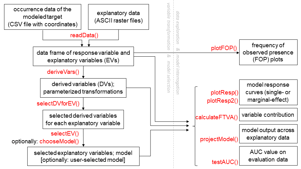
Workflow
The diagram below outlines a common workflow for users of the package. Function names are in red.
Author(s)
Maintainer: Julien Vollering julienvollering@gmail.com
Authors:
Sabrina Mazzoni
Rune Halvorsen
Other contributors:
Steven Phillips [copyright holder]
Michael Bedward [contributor]
References
Fithian, W., & Hastie, T. (2013). Finite-sample equivalence in statistical models for presence-only data. The annals of applied statistics, 7(4), 1917.
Halvorsen, R., Mazzoni, S., Bryn, A. & Bakkestuen, V. (2015) Opportunities for improved distribution modelling practice via a strict maximum likelihood interpretation of MaxEnt. Ecography, 38, 172-183.
Halvorsen, R., Mazzoni, S., Dirksen, J.W., Næsset, E., Gobakken, T. & Ohlson, M. (2016) How important are choice of model selection method and spatial autocorrelation of presence data for distribution modelling by MaxEnt? Ecological Modelling, 328, 108-118.
Mazzoni, S., Halvorsen, R. & Bakkestuen, V. (2015) MIAT: Modular R-wrappers for flexible implementation of MaxEnt distribution modelling. Ecological Informatics, 30, 215-221.
Phillips, S.J., Anderson, R.P., Dudík, M., Schapire, R.E., & Blair, M.E. (2017). Opening the black box: an open-source release of Maxent. Ecography, 40(7), 887-893.
Phillips, S.J., Anderson, R.P. & Schapire, R.E. (2006) Maximum entropy modeling of species geographic distributions. Ecological Modelling, 190, 231-259.
Vollering, J., Halvorsen, R., & Mazzoni, S. (2019) The MIAmaxent R package: Variable transformation and model selection for species distribution models. Ecology and Evolution, 9(21), 12051–12068.
See Also
Useful links:
Report bugs at https://github.com/julienvollering/MIAmaxent/issues
Calculates variable contributions as RVA
Description
Calculates the Relative Variation Accounted for (Halvorsen et al.
2015), for the selected model or a chosen model from the results of
selectEV.
Usage
calculateRVA(selectedEV, formula = NULL)
Arguments
selectedEV |
The list returned by |
formula |
If null, RVA is calculated for the selected model in
|
References
Halvorsen, R., Mazzoni, S., Bryn, A., & Bakkestuen, V. (2015). Opportunities for improved distribution modelling practice via a strict maximum likelihood interpretation of MaxEnt. Ecography, 38(2), 172-183.
Examples
## Not run:
# From vignette:
calculateRVA(grasslandEVselect, formula("~ prbygall + geoberg + lcucor1 +
tertpi09 + geolmja1"))

## End(Not run)
Trains a model containing the explanatory variables specified.
Description
chooseModel trains a model based on the formula provided. The formula
specifies which explanatory variables (EVs) — and potentially first-order
interactions between these — should be included in the model. Each EV can
be represented by 1 or more derived variables (see deriveVars).
The function may be employed to choose a model from the selection pathway of
selectEV other than the model selected under the provided alpha
value.
Usage
chooseModel(dvdata, formula, algorithm = "maxent")
Arguments
dvdata |
A list containing first the response variable, followed by data
frames of selected derived variables for a given explanatory
variable (e.g. the first item in the list returned by
|
formula |
A model formula (in the form y ~ x + ...) specifying the
independent terms (EVs) to be included in the model. The item in
|
algorithm |
Character string matching either "maxent" or "LR", which determines the type of model built. Default is "maxent". |
Details
Explanatory variables should be uniquely named. Underscores ('_') and colons
(':') are reserved to denote derived variables and interaction terms
respectively, and chooseModel will replace these — along with other
special characters — with periods ('.').
Examples
## Not run:
# From vignette:
grasslandmodel <- chooseModel(grasslandDVselect$dvdata,
                              formula("~ pr.bygall + geoberg + lcucor1 +
                                      tertpi09 + geolmja1"))

## End(Not run)
Derive variables by transformation.
Description
deriveVars produces derived variables from explanatory variables by
transformation, and returns a list of dataframes. The available
transformation types are as follows, described in Halvorsen et al. (2015): L,
M, D, HF, HR, T (for continuous EVs), and B (for categorical EVs). For spline
transformation types (HF, HR, T), a subset of possible DVs is pre-selected
by the criteria described under Details.
Usage
deriveVars(
  data,
  transformtype = c("L", "M", "D", "HF", "HR", "T", "B"),
  allsplines = FALSE,
  algorithm = "maxent",
  write = FALSE,
  dir = NULL,
  quiet = FALSE
)
Arguments
data |
Data frame containing the response variable in the first column
and explanatory variables in subsequent columns. The response variable
should represent either presence and background (coded as 1/NA) or presence
and absence (coded as 1/0). The explanatory variable data should be
complete (no NAs). See |
transformtype |
Specifies the types of transformations types to be performed. Default is the full set of the following transformation types: L (linear), M (monotone), D (deviation), HF (forward hinge), HR (reverse hinge), T (threshold), and B (binary). |
allsplines |
Logical. Keep all spline transformations created, rather than pre-selecting particular splines based on fraction of total variation explained. |
algorithm |
Character string matching either "maxent" or "LR", which determines the type of model used for spline pre-selection. See Details. |
write |
Logical. Write the transformation functions to .Rdata file?
Default is |
dir |
Directory for file writing if |
quiet |
Logical. Suppress progress messages from spline pre-selection? |
Details
The linear transformation "L" is a simple rescaling to the range [0, 1].
The monotone transformation "M" performed is a zero-skew transformation (Økland et al. 2001).
The deviation transformation "D" is performed around an optimum EV value that
is found by looking at frequency of presence (see plotFOP).
Three deviation transformations are created with different steepness and
curvature around the optimum.
For spline transformations ("HF", "HR", and "T"), DVs are created around 20 different break points (knots) which span the range of the EV. Only DVs which satisfy all of the following criteria are retained:
3 <= knot <= 18 (DVs with knots at the extremes of the EV are never retained).
Chi-square test of the single-variable model from the given DV compared to the null model gives a p-value < 0.05.
The single-variable model from the given DV shows a local maximum in fraction of variation explained (D^2, sensu Guisan & Zimmerman, 2000) compared to DVs from the neighboring 4 knots.
The models used in this pre-selection procedure may be maxent models (algorithm="maxent") or standard logistic regression models (algorithm="LR").
For categorical variables, 1 binary derived variable (type "B") is created for each category.
The maximum entropy algorithm ("maxent") — which is implemented in MIAmaxent as an infinitely-weighted logistic regression with presences added to the background — is conventionally used with presence-only occurrence data. In contrast, standard logistic regression (algorithm = "LR"), is conventionally used with presence-absence occurrence data.
Explanatory variables should be uniquely named. Underscores ('_') and colons
(':') are reserved to denote derived variables and interaction terms
respectively, and deriveVars will replace these — along with other
special characters — with periods ('.').
Value
List of 2:
dvdata: List containing first the response variable, followed data frames of derived variables produced for each explanatory variable. This item is recommended as input for
dvdatainselectDVforEV.transformations: List containing first the response variable, followed by all the transformation functions used to produce the derived variables.
References
Guisan, A., & Zimmermann, N. E. (2000). Predictive habitat distribution models in ecology. Ecological modelling, 135(2-3), 147-186.
Halvorsen, R., Mazzoni, S., Bryn, A., & Bakkestuen, V. (2015). Opportunities for improved distribution modelling practice via a strict maximum likelihood interpretation of MaxEnt. Ecography, 38(2), 172-183.
Økland, R.H., Økland, T. & Rydgren, K. (2001). Vegetation-environment relationships of boreal spruce swamp forests in Østmarka Nature Reserve, SE Norway. Sommerfeltia, 29, 1-190.
Examples
toydata_dvs <- deriveVars(toydata_sp1po, c("L", "M", "D", "HF", "HR", "T", "B"))
str(toydata_dvs$dvdata)
summary(toydata_dvs$transformations)

## Not run:
# From vignette:
grasslandDVs <- deriveVars(grasslandPO,
                           transformtype = c("L","M","D","HF","HR","T","B"))
summary(grasslandDVs$dvdata)
head(summary(grasslandDVs$transformations))
length(grasslandDVs$transformations)
plot(grasslandPO$terslpdg, grasslandDVs$dvdata$terslpdg$terslpdg_D2, pch=20,
     ylab="terslpdg_D2")
plot(grasslandPO$terslpdg, grasslandDVs$dvdata$terslpdg$terslpdg_M, pch=20,
     ylab="terslpdg_M")

## End(Not run)
Maxent model from .lambdas file.
Description
modelFromLambdas returns an R function for a given Maxent model, using
the .lambdas file produced by the MaxEnt program to parameterize the model.
The returned function gives predictions of the model in "raw output" format
from values of explanatory variables.
Usage
modelFromLambdas(file, raw = FALSE)
Arguments
file |
pathway to the .lambdas file of a given Maxent model |
raw |
Logical. Should the function return raw Maxent output instead of PRO? |
Details
The modelFromLambdas function returns a Maxent model, in the form of a
function that calculates Maxent predictions for given values of explanatory
variables.
Input to the function returned by modelFromLambdas are values of
explanatory variables in the model. The format of this input must be an array
(matrix or data frame) with m columns, and column names must match variable
names in the .lambdas file used to reproduce the model.
Value
returns an R function (object).
Plot Frequency of Observed Presence (FOP).
Description
plotFOP produces a Frequency of Observed Presence (FOP) plot for a
given explanatory variable. An FOP plot shows the rate of occurrence of the
response variable across intervals or levels of the explanatory variable. For
continuous variables, a local regression ("loess") of the FOP values is added
to the plot as a line. Data density is plotted in the background (grey) to
help visualize where FOP values are more or less certain.
Usage
plotFOP(
  data,
  EV,
  span = 0.5,
  intervals = NULL,
  ranging = FALSE,
  densitythreshold = NULL,
  ...
)
Arguments
data |
Data frame containing the response variable in the first column
and explanatory variables in subsequent columns. The response variable
should represent either presence and background (coded as 1/NA) or presence
and absence (coded as 1/0). See Details for information regarding
implications of occurrence data type. See also |
EV |
Name or column index of the explanatory variable in |
span |
The proportion of FOP points included in the local regression neighborhood. Should be between 0 and 1. Irrelevant for categorical EVs. |
intervals |
Number of intervals into which the continuous EV is divided. Defaults to the minimum of N/10 and 100. Irrelevant for categorical EVs. |
ranging |
Logical. If |
densitythreshold |
Numeric. Intervals containing fewer than this number of observations will be represented with an open symbol in the plot. Irrelevant for categorical EVs. |
... |
Arguments to be passed to
|
Details
A list of the optimum EV value and a data frame containing the plotted data is returned invisibly. Store invisibly returned output by assigning it to an object.
In the local regression ("loess"), the plotted FOP values are regressed against their EV values. The points are weighted by the number of observations they represent, such that an FOP value from an interval with many observations is given more weight.
For continuous variables, the returned value of 'EVoptimum' is based on the loess-smoothed FOP values, such that a point maximum in FOP may not always be considered the optimal value of EV.
If the response variable in data represents presence/absence data, the
result is an empirical frequency of presence curve, rather than a observed
frequency of presence curve (see Støa et al. [2018], Sommerfeltia).
Value
In addition to the graphical output, a list of 2:
-
EVoptimum. The EV value (or level, for categorical EVs) at which FOP is highest -
FOPdata. A data frame containing the plotted data. Columns in this data frame represent the following: EV interval ("int"), number of observations in the interval ("n"), mean EV value of the observations in the interval ("intEV"), mean RV value of the observations in the interval ("intRV"), and local regression predicted intRV ("loess"). For categorical variables, only the level name ("level"), the number of observations in the level ("n"), and the mean RV value of the level ("levelRV") are used.
References
Støa, B., R. Halvorsen, S. Mazzoni, and V. I. Gusarov. (2018). Sampling bias in presence-only data used for species distribution modelling: theory and methods for detecting sample bias and its effects on models. Sommerfeltia 38:1–53.
Examples
FOPev11 <- plotFOP(toydata_sp1po, 2)
FOPev12 <- plotFOP(toydata_sp1po, "EV12", intervals = 8)
FOPev12$EVoptimum
FOPev12$FOPdata

## Not run:
# From vignette:
teraspifFOP <- plotFOP(grasslandPO, "teraspif")
terslpdgFOP <- plotFOP(grasslandPO, "terslpdg")
terslpdgFOP <- plotFOP(grasslandPO, "terslpdg", span = 0.75, intervals = 20)
terslpdgFOP
geobergFOP <- plotFOP(grasslandPO, 10)
geobergFOP

## End(Not run)
Plot model response.
Description
Plots the response of a given model over any of the explanatory variables
(EVs) included in that model. For categorical variables, a bar plot is
returned rather than a line plot. Single-effect response curves show the
response of a model containing the explanatory variable of interest only,
while marginal effect response curves show the response of the model when all
other explanatory variables are held constant at their mean values (cf.
plotResp, plotResp2).
Usage
plotResp(model, transformations, EV, logscale = FALSE, ...)

plotResp2(model, transformations, EV, logscale = FALSE, ...)
Arguments
model |
The model for which the response is to be plotted. This may be
the object returned by |
transformations |
Transformation functions used to create the derived
variables in the model. I.e. the 'transformations' returned by
|
EV |
Character. Name of the explanatory variable for which the response curve is to be plotted. Interaction terms not allowed. |
logscale |
Logical. Plot the common logarithm of PRO rather than PRO itself. |
... |
Arguments to be passed to
|
Functions
-
plotResp(): Plot single-effect model response. -
plotResp2(): Plot marginal-effect model response.
Examples
## Not run:
# From vignette:
plotResp(grasslandmodel, grasslandDVs$transformations, "pr.bygall")
plotResp(grasslandmodel, grasslandDVs$transformations, "geolmja1")

plotResp2(grasslandmodel, grasslandDVs$transformations, "pr.bygall")

## End(Not run)
Predict method for infinitely-weighted logistic regression
Description
Returns model predictions for new data in "PRO" or "raw" format.
Usage
## S3 method for class 'MIAmaxent_iwlr'
predict(object, newdata, type = "PRO", ...)
Arguments
object |
Model of class "MIAmaxent_iwlr" |
newdata |
Data frame containing variables with which to predict |
type |
Type of model output: "PRO" or "raw" |
Project model across explanatory data.
Description
projectModel calculates model predictions for any points where values
of the explanatory variables in the model are known. It can be used to get
model predictions for the training data, or to project the model to a new
space or time.
Usage
projectModel(
  model,
  transformations,
  data,
  clamping = FALSE,
  raw = FALSE,
  rescale = FALSE,
  filename = NULL
)
Arguments
model |
The model to be projected. This may be the object returned by
|
transformations |
Transformation functions used to create the derived
variables in the model. I.e. the 'transformations' returned by
|
data |
Data frame of all the explanatory variables (EVs) included in the
model (see |
clamping |
Logical. Do clamping sensu Phillips et al. (2006).
Default is |
raw |
Logical. Return raw maxent output instead of probability ratio output (PRO)? Default is FALSE. Irrelevant for "LR"-type models. |
rescale |
Logical. Linearly rescale model output (PRO or raw) with
respect to the projection |
filename |
Full file pathway to write raster model predictions if
|
Details
Missing data (NA) for a continuous variable will result in NA output for that point. Missing data for a categorical variable is treated as belonging to none of the categories.
When rescale = FALSE the scale of the maxent model output (PRO or raw)
returned by this function is dependent on the data used to train the model.
For example, a location with PRO = 2 can be interpreted as having a
probability of presence twice as high as an average site in the
training data (Halvorsen, 2013, Halvorsen et al., 2015). When
rescale = TRUE, the output is linearly rescaled with respect to the
data onto which the model is projected. In this case, a location with PRO = 2
can be interpreted as having a probability of presence twice as high as an
average site in the projection data. Similarly, raw values are on a
scale which is dependent on the size of either the training data extent
(rescale = FALSE) or projection data extent (rescale = TRUE).
Value
List of 2:
output: A data frame with the model output in column 1 and the corresponding explanatory data in subsequent columns, or a raster containing predictions if
datais a SpatRaster.ranges: A list showing the range of
datacompared to the training data, on a 0-1 scale.
If data is a SpatRaster, the output
is also plotted.
References
Halvorsen, R. (2013) A strict maximum likelihood explanation of MaxEnt, and some implications for distribution modelling. Sommerfeltia, 36, 1-132.
Halvorsen, R., Mazzoni, S., Bryn, A. & Bakkestuen, V. (2015) Opportunities for improved distribution modelling practice via a strict maximum likelihood interpretation of MaxEnt. Ecography, 38, 172-183.
Phillips, S.J., Anderson, R.P. & Schapire, R.E. (2006) Maximum entropy modeling of species geographic distributions. Ecological Modelling, 190, 231-259.
Examples
## Not run:
# From vignette:
EVfiles <- c(list.files(system.file("extdata", "EV_continuous", package="MIAmaxent"),
                        full.names=TRUE),
             list.files(system.file("extdata", "EV_categorical", package="MIAmaxent"),
                        full.names=TRUE))
EVstack <- rast(EVfiles)
names(EVstack) <- gsub(".asc", "", basename(EVfiles))
grasslandPreds <- projectModel(model = grasslandmodel,
                               transformations = grasslandDVs$transformations,
                               data = EVstack)
grasslandPreds

## End(Not run)
Read in data object from files.
Description
readData reads in occurrence data in CSV file format and environmental
data in ASCII or GeoTIFF raster file format and produces a data object which
can be used as the starting point for the functions in this package. This
function is intended to make reading in data easy for users familiar with the
maxent.jar program. It is emphasized that important considerations for data
preparation (e.g. cleaning, sampling bias removal, etc.) are not treated in
this package and must be dealt with separately!
Usage
readData(
  occurrence,
  contEV = NULL,
  catEV = NULL,
  maxbkg = 10000,
  PA = FALSE,
  XY = FALSE,
  duplicates = FALSE
)
Arguments
occurrence |
Full pathway of the '.csv' file of occurrence data. The first column of the CSV should code occurrence (see Details), while the second and third columns should contain X and Y coordinates corresponding to the raster coordinate system. The first row of the csv is read as a header row. |
contEV |
Pathway to a directory containing continuous environmental variables in either '.asc' (ASCII) or '.tif' (GeoTIFF) file format. |
catEV |
Pathway to a directory containing categorical environmental variables in either '.asc' (ASCII) or '.tif' (GeoTIFF) file format. |
maxbkg |
Integer. Maximum number of grid cells randomly selected as
uninformed background locations for the response variable. Default is
10,000. Irrelevant for presence/absence data ( |
PA |
Logical. Does |
XY |
Logical. Include XY coordinates in the output. May be useful for spatial plotting. Note that coordinates included in the training data used to build the model will be treated as explanatory variables. |
duplicates |
Logical. Include each coordinate in |
Details
When occurrence represents presence-only data (PA = FALSE), all
rows with values other than 'NA' in column 1 of the CSV file are treated as
presence locations. If column 1 contains any values of 'NA', these rows are
treated as the uninformed background locations. Thus, 'NA' can be used to
specify a specific set of uninformed background locations if desired.
Otherwise uninformed background locations are randomly selected from the full
extent of the raster cells which are not already included as presence
locations. Only cells which contain data for all environmental variables are
retained as presence locations or selected as uninformed background
locations.
When occurrence represents presence/absence data (PA = TRUE),
rows with value '0' in column 1 of the CSV are treated as absence locations,
rows with value 'NA' are excluded, and all other rows are treated as
presences. If duplicates = FALSE, raster cells containing both
presence and absence locations result in a single presence row.
The names of the input raster files are used as the names of the explanatory
variables, so these files should be uniquely named. readData replaces
underscores '_', spaces ' ' and other special characters not allowed in names
with periods '.'. In MIAmaxent, underscores and colons are reserved to denote
derived variables and interaction terms, respectively.
Value
Data frame with the Response Variable (RV) in the first column, and
Explanatory Variables (EVs) in subsequent columns. When PA = FALSE,
RV values are 1/NA, and when PA = TRUE, RV values are 1/0.
Examples
toydata_sp1po <- readData(system.file("extdata/sommerfeltia", "Sp1.csv", package = "MIAmaxent"),
   contEV = system.file("extdata/sommerfeltia", "EV_continuous", package = "MIAmaxent"))
toydata_sp1po

## Not run:
# From vignette:
grasslandPO <- readData(
 occurrence=system.file("extdata", "occurrence_PO.csv", package="MIAmaxent"),
  contEV=system.file("extdata", "EV_continuous", package="MIAmaxent"),
  catEV=system.file("extdata", "EV_categorical", package="MIAmaxent"),
  maxbkg=20000)
str(grasslandPO)

# From vignette:
grasslandPA <- readData(
  occurrence = system.file("extdata", "occurrence_PA.csv", package="MIAmaxent"),
  contEV = system.file("extdata", "EV_continuous", package="MIAmaxent"),
  catEV = system.file("extdata", "EV_categorical", package="MIAmaxent"),
  PA = TRUE, XY = TRUE)
head(grasslandPA)
tail(grasslandPA)

## End(Not run)
Select parsimonious sets of derived variables.
Description
For each explanatory variable (EV), selectDVforEV selects the
parsimonious set of derived variables (DV) which best explains variation in a
given response variable. The function uses a process of forward selection
based on comparison of nested models using inference tests. A DV is selected
for inclusion when, during nested model comparison, it accounts for a
significant amount of remaining variation, under the alpha value specified by
the user. See Halvorsen et al. (2015) for a more detailed explanation of the
forward selection procedure.
Usage
selectDVforEV(
  dvdata,
  alpha = 0.01,
  retest = FALSE,
  test = "Chisq",
  algorithm = "maxent",
  write = FALSE,
  dir = NULL,
  quiet = FALSE
)
Arguments
dvdata |
List containing first the response variable, followed by data
frames of derived variables produced for each explanatory variable (e.g.
the first item in the list returned by |
alpha |
Alpha-level used for inference testing in nested model comparison. Default is 0.01. |
retest |
Logical. Test variables that do not meet the alpha criterion
in a given round in subsequent rounds? Default is |
test |
Character string matching either "Chisq" or "F" to determine which inference test is used in nested model comparison. The Chi-squared test is implemented by stats::anova, while the F-test is implemented as described in Halvorsen (2013, 2015). Default is "Chisq". |
algorithm |
Character string matching either "maxent" or "LR", which determines the type of model used during forward selection. Default is "maxent". |
write |
Logical. Write the trail of forward selection for each EV to
.csv file? Default is |
dir |
Directory for file writing if |
quiet |
Suppress progress bar? |
Details
The F-test available in selectDVforEV is calculated using equation 59
in Halvorsen (2013).
If using binary-type derived variables from deriveVars, be
aware that a model including all of these DVs will be considered equal to the
the closest nested model, due to perfect multicollinearity (i.e. the dummy
variable trap).
The maximum entropy algorithm ("maxent") — which is implemented in MIAmaxent as an infinitely-weighted logistic regression with presences added to the background — is conventionally used with presence-only occurrence data. In contrast, standard logistic regression (algorithm = "LR"), is conventionally used with presence-absence occurrence data.
Explanatory variables should be uniquely named. Underscores ('_') and colons
(':') are reserved to denote derived variables and interaction terms
respectively, and selectDVforEV will replace these — along with
other special characters — with periods ('.').
Value
List of 2:
dvdata: A list containing first the response variable, followed by data frames of selected DVs for each EV. EVs with zero selected DVs are dropped. This item is recommended as input for
dvdatainselectEV.selection: A list of data frames, where each data frame shows the trail of forward selection of DVs for a given EV.
References
Halvorsen, R. (2013). A strict maximum likelihood explanation of MaxEnt, and some implications for distribution modelling. Sommerfeltia, 36, 1-132.
Halvorsen, R., Mazzoni, S., Bryn, A., & Bakkestuen, V. (2015). Opportunities for improved distribution modelling practice via a strict maximum likelihood interpretation of MaxEnt. Ecography, 38(2), 172-183.
Examples
toydata_seldvs <- selectDVforEV(toydata_dvs$dvdata, alpha = 0.4)

## Not run:
# From vignette:
grasslandDVselect <- selectDVforEV(grasslandDVs$dvdata, alpha = 0.001)
summary(grasslandDVs$dvdata)
sum(sapply(grasslandDVs$dvdata[-1], length))
summary(grasslandDVselect$dvdata)
sum(sapply(grasslandDVselect$dvdata[-1], length))
grasslandDVselect$selection$terdem

## End(Not run)
Select parsimonious set of explanatory variables.
Description
selectEV selects the parsimonious set of explanatory variables (EVs)
which best explains variation in a given response variable (RV). Each EV can
be represented by 1 or more derived variables (see deriveVars
and selectDVforEV). The function uses a process of forward
selection based on comparison of nested models using inference tests. An EV
is selected for inclusion when, during nested model comparison, it accounts
for a significant amount of remaining variation, under the alpha value
specified by the user. See Halvorsen et al. (2015) for a more detailed
explanation of the forward selection procedure.
Usage
selectEV(
  dvdata,
  alpha = 0.01,
  retest = FALSE,
  interaction = FALSE,
  formula = NULL,
  test = "Chisq",
  algorithm = "maxent",
  write = FALSE,
  dir = NULL,
  quiet = FALSE
)
Arguments
dvdata |
List containing first the response variable, followed by data
frames of selected derived variables for a given explanatory
variable (e.g. the first item in the list returned by
|
alpha |
Alpha-level used in F-test comparison of models. Default is 0.01. |
retest |
Logical. Test variables (or interaction terms) that do not meet
the alpha criterion in a given round in subsequent rounds? Default is
|
interaction |
Logical. Allow interaction terms between pairs of EVs?
Default is |
formula |
A model formula (in the form y ~ x + ...) specifying a
starting point for forward model selection. The independent terms in the
formula will be included in the model regardless of explanatory power, and
must be represented in |
test |
Character string matching either "Chisq" or "F" to determine which inference test is used in nested model comparison. The Chi-squared test is implemented by stats::anova, while the F-test is implemented as described in Halvorsen (2013, 2015). Default is "Chisq". |
algorithm |
Character string matching either "maxent" or "LR", which determines the type of model used during forward selection. Default is "maxent". |
write |
Logical. Write the trail of forward selection to .csv file?
Default is |
dir |
Directory for file writing if |
quiet |
Logical. Suppress progress messages from EV-selection? |
Details
The F-test available in selectEV is calculated using equation 59 in
Halvorsen (2013).
When interaction = TRUE, the forward selection procedure selects a
parsimonious group of individual EVs first, and then tests interactions
between EVs included in the model afterwards. Therefore, interactions are
only explored between terms which are individually explain a significant
amount of variation. When interaction = FALSE, interactions are not
considered. Practically, interactions between EVs are represented by the
products of all combinations of their component DVs (Halvorsen, 2013).
The maximum entropy algorithm ("maxent") — which is implemented in MIAmaxent as an infinitely-weighted logistic regression with presences added to the background — is conventionally used with presence-only occurrence data. In contrast, standard logistic regression (algorithm = "LR"), is conventionally used with presence-absence occurrence data.
Explanatory variables should be uniquely named. Underscores ('_') and colons
(':') are reserved to denote derived variables and interaction terms
respectively, and selectEV will replace these — along with other
special characters — with periods ('.').
Value
List of 3:
dvdata: A list containing first the response variable, followed by data frames of DVs for each selected EV.
selection: A data frame showing the trail of forward selection of individual EVs (and interaction terms if necessary).
selectedmodel: the selected model under the given alpha value.
References
Halvorsen, R. (2013). A strict maximum likelihood explanation of MaxEnt, and some implications for distribution modelling. Sommerfeltia, 36, 1-132.
Halvorsen, R., Mazzoni, S., Bryn, A., & Bakkestuen, V. (2015). Opportunities for improved distribution modelling practice via a strict maximum likelihood interpretation of MaxEnt. Ecography, 38(2), 172-183.
Examples
## Not run:
# From vignette:
grasslandEVselect <- selectEV(grasslandDVselect$dvdata, alpha = 0.001,
                              interaction = TRUE)
summary(grasslandDVselect$dvdata)
length(grasslandDVselect$dvdata[-1])
summary(grasslandEVselect$dvdata)
length(grasslandEVselect$dvdata[-1])
grasslandEVselect$selectedmodel$formula

## End(Not run)
Calculate model AUC with test data.
Description
For a given model, testAUC calculates the Area Under the Curve (AUC)
of the Receiver Operating Characteristic (ROC) as a threshold-independent
measure of binary classification performance. This function is intended to be
used with occurrence data that is independent from the data used to train the
model, to obtain an unbiased measure of model performance.
Usage
testAUC(model, transformations, data, plot = TRUE, ...)
Arguments
model |
The model to be projected. This may be the object returned by
|
transformations |
Transformation functions used to create the derived
variables in the model. I.e. the 'transformations' returned by
|
data |
Data frame containing test occurrence data in the first column
and corresponding explanatory variables in the model in subsequent columns.
The test data should be coded as: 1/0/NA, representing presence, absence,
and uninformed. See |
plot |
Logical. Plot the ROC curve? |
... |
Arguments to be passed to
Note that some graphical parameters may return errors or warnings if they cannot be changed or correspond to multiple elements in the plot. |
Details
If plotted, the point along the ROC curve where the discrimination threshold is PRO = 1, is shown for reference.
Examples
## Not run:
# From vignette:
grasslandPA <- readData(
  occurrence = system.file("extdata", "occurrence_PA.csv", package="MIAmaxent"),
  contEV = system.file("extdata", "EV_continuous", package="MIAmaxent"),
  catEV = system.file("extdata", "EV_categorical", package="MIAmaxent"),
  PA = TRUE, XY = TRUE)
head(grasslandPA)
tail(grasslandPA)
testAUC(model = grasslandmodel, transformations = grasslandDVs$transformations,
        data = grasslandPA)

## End(Not run)
Derived variables and transformation functions, from toy data.
Description
Derived variables and transformation functions for distribution modeling of a small, synthetic data set used in Halvorsen (2013).
Usage
toydata_dvs
Format
List with 2 elements:
A list of 5, with the response variable followed by data frames each containing the derived variables produced for a given explanatory variable.
A list of the response variable and all the transformation functions used to produce the derived variables.
Source
Produced from toydata_sp1po using
deriveVars.
References
Halvorsen, R. (2013) A strict maximum likelihood explanation of MaxEnt, and some implications for distribution modelling. Sommerfeltia, 36, 1-132.
Selected derived variables accompanied by selection trails, from toy data.
Description
Selected derived variables and tables showing forward model selection of derived variables for distribution modeling of a small, synthetic data set used in Halvorsen (2013).
Usage
toydata_seldvs
Format
List with 2 elements:
A list of 3, with the response variable followed by data frames each containing the derived variables selected for a given explanatory variable.
A list of the response variable and forward model selection trails used to select derived variables.
Source
Produced from toydata_dvs using
selectDVforEV.
References
Halvorsen, R. (2013) A strict maximum likelihood explanation of MaxEnt, and some implications for distribution modelling. Sommerfeltia, 36, 1-132.
Selected explanatory variables accompanied by selection trails, from toy data.
Description
Selected explanatory variables and tables showing forward model selection of explanatory variables for distribution modeling of a small, synthetic data set used in Halvorsen (2013). Each individual explanatory variable is represented by a group of derived variables.
Usage
toydata_selevs
Format
List with 3 elements:
A list of 3, with the response variable followed by data frames, represent selected explanatory variables.
A trail of forward model selection used to select explanatory variables and interaction terms.
The selected model
Source
Produced from toydata_seldvs using
selectEV.
References
Halvorsen, R. (2013) A strict maximum likelihood explanation of MaxEnt, and some implications for distribution modelling. Sommerfeltia, 36, 1-132.
Occurrence and environmental toy data.
Description
A small, synthetic data set for distribution modeling, consisting of occurrence and environmental data, from Halvorsen (2013). The study area consists of 40 grid cells, with 8 row and 5 columns, in which 10 presences occur.
Usage
toydata_sp1po
Format
A data frame with 40 rows and 5 variables:
- RV
response variable, occurrence either presence or uninformed background
- EV11
explanatory variable: northing
- EV12
explanatory variable: easting
- EV13
explanatory variable: modified random uniform
- EV14
explanatory variable: random uniform
Source
Halvorsen, R. (2013) A strict maximum likelihood explanation of MaxEnt, and some implications for distribution modelling. Sommerfeltia, 36, 1-132.